When managing approvals, budgets, or expenses in Google Sheets, it’s common to track items using checkboxes. For example, you might have a list of reimbursements where a checkbox in the “Approved” column indicates whether the expense is approved. In such cases, you may want to calculate the total amount of approved entries only.
In this article, we’ll explore four effective methods to sum values based on whether a checkbox is checked (TRUE) or unchecked (FALSE). Using a real-world example of employee expense reports, you’ll learn how to apply the SUMIFS function, the FILTER and SUM functions, the ARRAYFORMULA and IF functions, and the QUERY function to calculate totals based on checkbox status.
Steps to sum amounts only when checkboxes are checked using SUMIFS in Google Sheets:
➤ Select a blank cell for the result (e.g., C10).
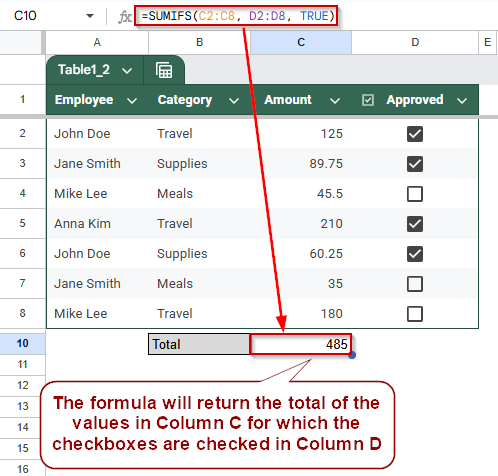
➤ In cell C10, enter this formula:
=SUMIFS(C2:C8, D2:D8, TRUE)
➤ Press Enter to calculate the total of only approved entries.
➤ The formula dynamically sums values in the “Amount” column where the “Approved” checkbox is TRUE.
Use SUMIFS to Sum Amounts If Checkbox Is Checked in Google Sheets
The SUMIFS function is one of the easiest ways to calculate totals based on specific conditions. In this case, we’ll use it to sum only those rows where the checkbox in the “Approved” column is checked (TRUE). This is a common need in budgeting sheets, reimbursement logs, or approval workflows.
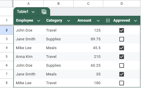
We will be using this dataset to demonstrate the methods:
After applying this method, you’ll get the total amount of all approved expenses, without needing to filter or hide data manually.
Steps:
➤ Select the cell where you want the total (e.g., C10).
➤ Enter the following formula:
=SUMIFS(C2:C8, D2:D8, TRUE)
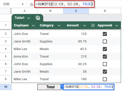
➧ D2:D8 is the Approved column with checkboxes (TRUE or FALSE).
➧ TRUE tells the formula to only include rows where the checkbox is checked.
➤ Press Enter.

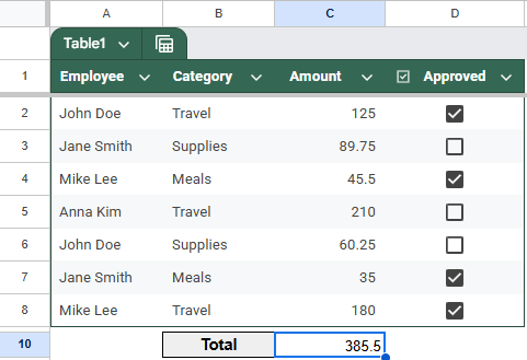
The total will dynamically change whenever you check or uncheck the boxes in Column D.
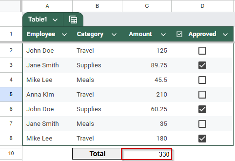
The result will display the sum of amounts for all approved entries, a clean and accurate total with no need for filtering or extra columns.
Utilize FILTER & SUM to Sum Amounts When Checkbox Is Checked in Google Sheets
The FILTER function can extract only the rows that meet specific criteria, like having the “Approved” checkbox checked. By combining FILTER with SUM, you can dynamically sum just the approved amounts.
After applying this method, you’ll get the total of all amounts where the approval checkbox is TRUE, giving you a flexible way to sum filtered data without extra columns.
Steps:
➤ Click on the cell where you want to display the total sum of approved amounts (for example, C10).
➤ Type the following formula exactly:
=SUM(FILTER(C2:C8, D2:D8=TRUE))
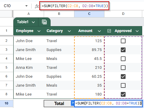
➧ SUM(...) adds all the filtered amounts to return the total approved sum.
➤ Press Enter to apply the formula.
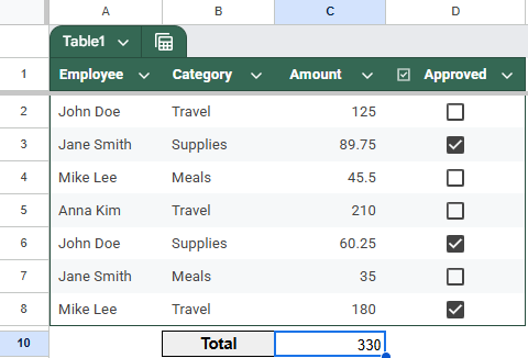
The formula will sum only the values in the Amount column (C2:C8) where the corresponding Approved checkbox in column D (D2:D8) is checked (TRUE).
➤ If you add more rows or change the checkboxes, the total will update automatically.
This method is perfect for summing data based on checkboxes without needing helper columns or complicated formulas. It’s clean, dynamic, and easy to maintain.
Combine ARRAYFORMULA with IF to Sum Amounts When Checkbox Is Checked
This method uses ARRAYFORMULA combined with IF to create a dynamic, row-by-row check of the Approved column. It multiplies the amounts by TRUE/FALSE values, treating TRUE as 1 and FALSE as 0, then sums the results. This approach automatically adjusts as you add or update data.
After applying this formula, you’ll get the total sum of all approved amounts, updated instantly when checkboxes change.
Steps:
➤ Select the cell where you want the total approved amount to appear (e.g., C10).
➤ Enter this formula:
=SUM(ARRAYFORMULA(IF(D2:D8=TRUE, C2:C8, 0)))
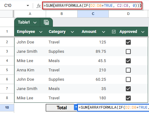
➧ ARRAYFORMULA(...) applies this check across the whole range without needing to copy the formula down each row.
➧ SUM(...) adds all the filtered amounts, returning the total approved sum.
➤ Press Enter to apply the formula.

➤ This formula automatically updates as you check or uncheck boxes or add more data within the specified range.

This method provides a clean, formula-driven way to dynamically calculate totals based on checkboxes, without helper columns or extra steps. It’s especially useful for datasets where rows are frequently added or updated.
Sum Values If Checkbox Is Checked Using the QUERY Function
The QUERY function lets you apply powerful SQL-like commands to your data, making it easy to filter and sum amounts based on checkbox status. This method sums all amounts where the Approved column is TRUE by querying your dataset dynamically.
After applying this method, you will see a clean summary showing the total sum of approved amounts without needing extra columns or complicated formulas.
Steps:
➤ Select the cell where you want the result to appear (e.g., F1).
➤ Enter the following formula:
=QUERY(A1:D8, “SELECT SUM(C) WHERE D = TRUE LABEL SUM(C) ‘Total Approved Amount'”, 1)
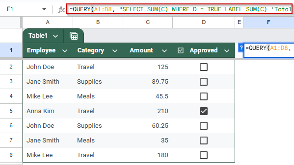
➧ SELECT SUM(C) WHERE D = TRUE tells QUERY to sum values in column C where the Approved column D is TRUE.
➧ LABEL SUM(C) Total Approved Amount renames the output column header for clarity.
➧ The final 1 indicates that the first row contains headers.
➤ Press Enter to run the query.
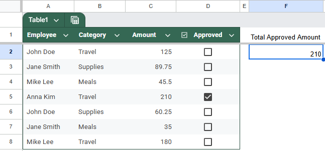
The formula scans the range A1:D8, selecting rows where the Approved column (D) is TRUE, and sums the corresponding Amount values from column C.. The result will be displayed as a single cell showing the total approved amount with a clear header “Total Approved Amount.”
➤ The total amount will dynamically change as you click on the checkboxes.

Frequently Asked Questions
How do I sum values based on a checked checkbox in Google Sheets?
Use =SUMIF(range_checkbox, TRUE, range_values) to sum amounts where the checkbox column is TRUE. It sums only the rows with checked boxes efficiently.
Why is my SUMIF not working with checkboxes?
Check that checkboxes return TRUE/FALSE, not text. Also, ensure ranges are the same size and formatted properly. Using SUMPRODUCT with (checkbox_range) can help as an alternative.
Can I sum with multiple conditions including a checkbox in Google Sheets?
Yes! Use SUMIFS with criteria like SUMIFS(amount_range, checkbox_range, TRUE, other_range, “criteria”) to sum only checked rows that meet extra conditions.
How to sum values dynamically with checkboxes using ARRAYFORMULA?
Combine ARRAYFORMULA with IF like =ARRAYFORMULA(SUM(IF(checkbox_range, amount_range, 0))) to sum values for checked boxes without dragging formulas down.
Wrapping Up
Summing amounts based on checked checkboxes in Google Sheets is easy with the right formula. Whether you prefer the straightforward SUMIFS function, the flexible FILTER and SUM method, the dynamic ARRAYFORMULA and IF approach, or the powerful QUERY function, each method helps you efficiently calculate totals only for approved entries. Select the one that best fits your workflow, and maintain clean and accurate data analysis with these straightforward, effective techniques.