Multiple dependent dropdown lists in Google Sheets is a useful feature you should learn. For example, you are making a sheet where users will first select a city, and then, based on that city, they will select a school.
But without dependent dropdowns, the person who is entering data might choose the wrong combination, like a Sydney school under Perth city.
If you use dependent dropdown lists correctly, Google Sheets only shows valid options based on the option you selected first.
In this article, we’ll show you how to set that up with a manual method that works. Let’s begin.
Summary of the steps to create multi-level dependent drop down list in Google Sheets:
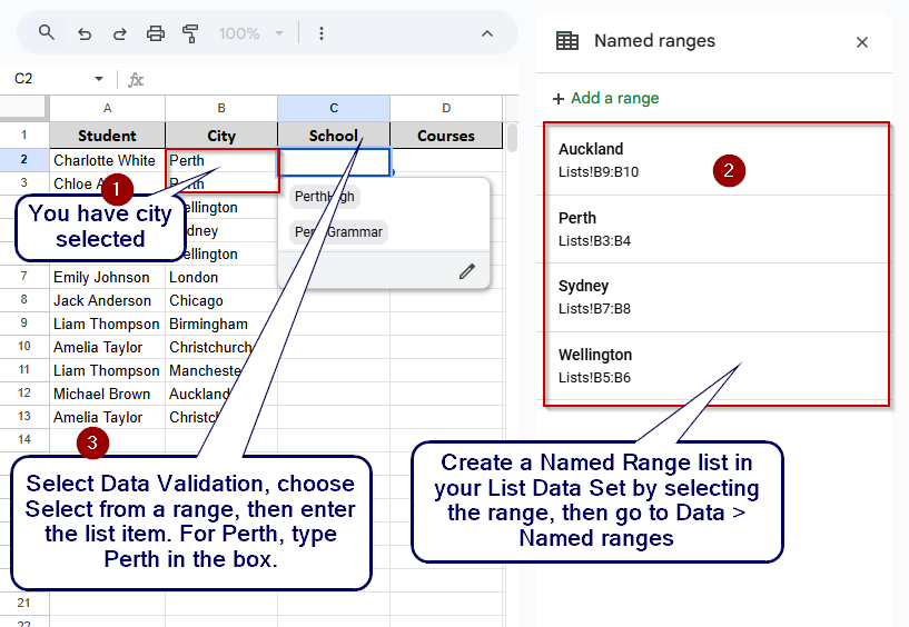
➤ We have a city selected the Column B where we have a city name.
➤ We want to show schools based on the city in Column C.
Prepare the list sheet:
➤ Make another sheet (let’s say it’s named List).
➤ Make a City to School list where you will write the name of the city and the schools for each city.
Create named ranges:
➤ Select the school list under each city name one by one.
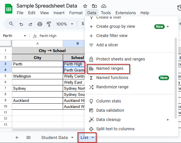
➤ Go to Data > Named ranges (from the Menu Bar).
➤ Name each range using the exact city name.
Apply dependent dropdown:
➤ Go back to the main sheet. Select the first cell in Column C where you want the school dropdown to appear.
➤ Go to Data > Data validation.
➤ Set Criteria to “Dropdown (from a range)”
➤ Type the named range manually, like =Perth, if the city selected in Column B is Perth.
➤ That cell will now only show schools under Perth.
➤ You have to repeat the same step manually for each row.
Steps to Add or Create Multiple Dependent Drop-down List in Google Sheets
In the following dataset, we have a list of students in Column A and their cities in Column B. In Column C, we want to select a school based on the selected city. And in Column D, we want to choose a course based on the selected school.
So, we have to create multiple drop-downs in Google Sheets to achieve that. The formation will be. City → School → Course.
Here is our sample dataset with which we will work.
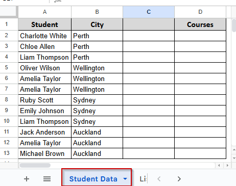
Step 1: Create the Main Dataset
➤ Create a sheet named “Student list” and enter the data set as shown in the previous screenshot.
Step 2: Create Another Backend Sheet and name it List.
We’re going to create multiple dependent dropdown lists in Google Sheets.
Here’s what we want to achieve:
Column B in the student sheet already contains the City names.
Column C → School will be a dropdown that depends on the City in Column B.
Column D → Course will be a dropdown that depends on the selected School in Column C.
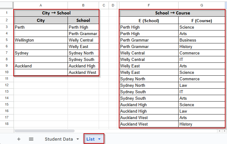
We will have to create a backend sheet to make this work. Here is how we organized them:
➤ Column A → City
➤ Column B → School (based on City)
➤ Column F → School
➤ Column G → Course (based on School)
Step 3: Define Named Ranges for Each Category
Now that we have the list table in place, we need to define Named Ranges so that we can use them in our dropdown settings.
Here’s what we will do:
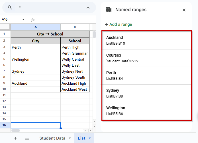
➤ First, go to the List sheet where we’ve prepared the City → School, and School → Course data.
➤ Select the cells B3:B4. We selected these two because these two schools located in Perth.
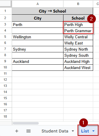
➤ From the top menu, go to Data → Named ranges.
➤ Now you will see the Name ranges Option Column appear on the right side of your screen.
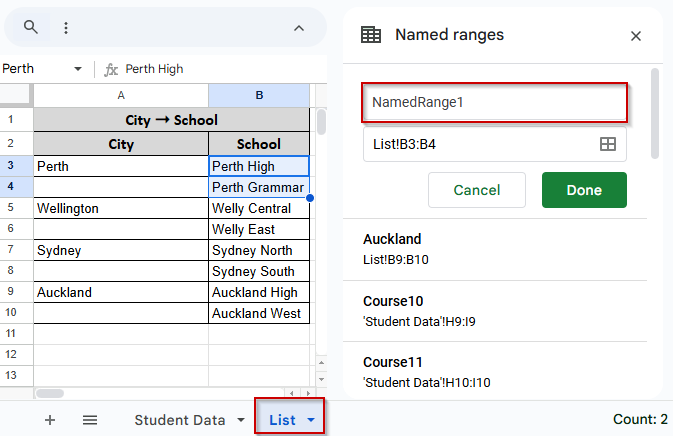
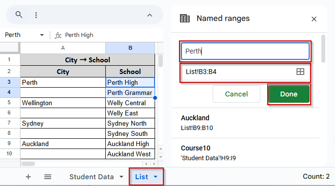
➤ You can see two boxes. In the First Box, write “Perth.”
➤ No need to write anything in the second box, as we have already selected B3:B4 cells.
➤ Now click on Done.
➤ You will see that a Name Range is created.
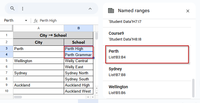
➤ Do the same for the rest of the cities. After finishing, you will create 4 name ranges like the following screenshot.
Step 4: Create the School Drop-down List in the Student List Sheet
Now that we’ve created our Named Ranges, it’s time to use them to build our first dependent drop-down list. We will use them to create the School drop-down in Column C based on the selected City in Column B.
Here’s how:
➤ Go to the “Student list” sheet.
➤ Select the first cell under the School column. In our case, it is C2.
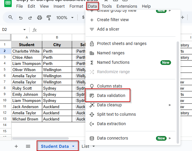
➤ From the top menu, click on Data → Data validation.
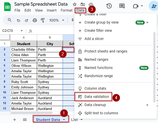
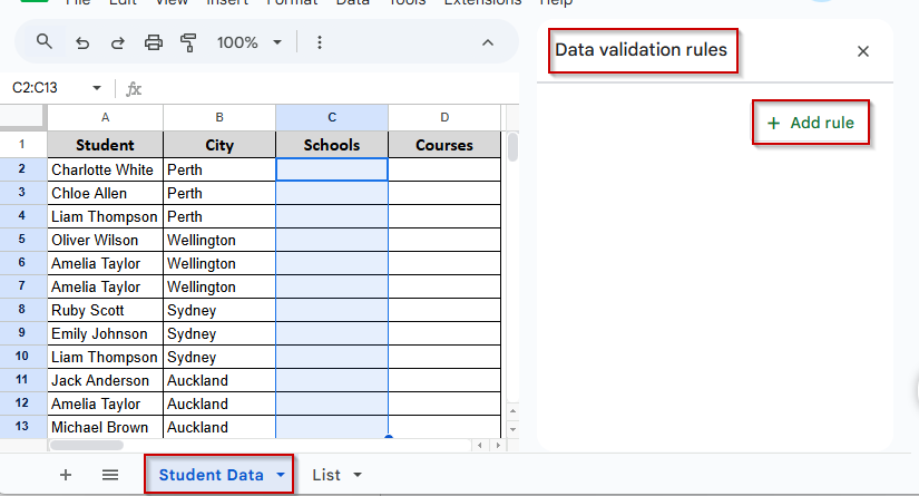
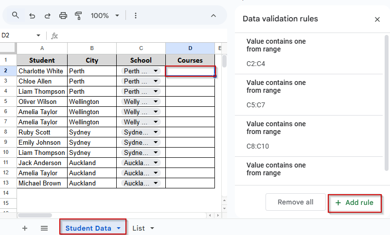
➤ Now you’ll see the Data validation panel on the right side of your screen.
➤ Click on Add Rule.
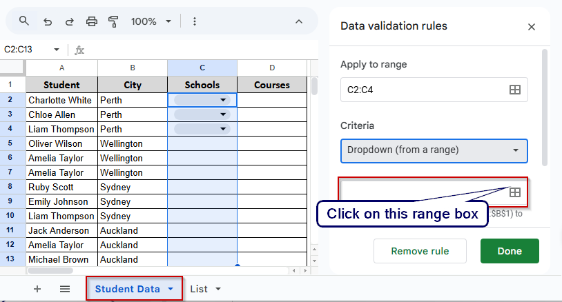
➤ In the Apply to Range box, write C2:C4. It’s because we have 3 schools in Perth. Look at Column B.
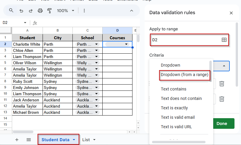
➤ Then, in the Criteria section, select Dropdown (from a range). You will see some drop-down boxes appear in Column C.
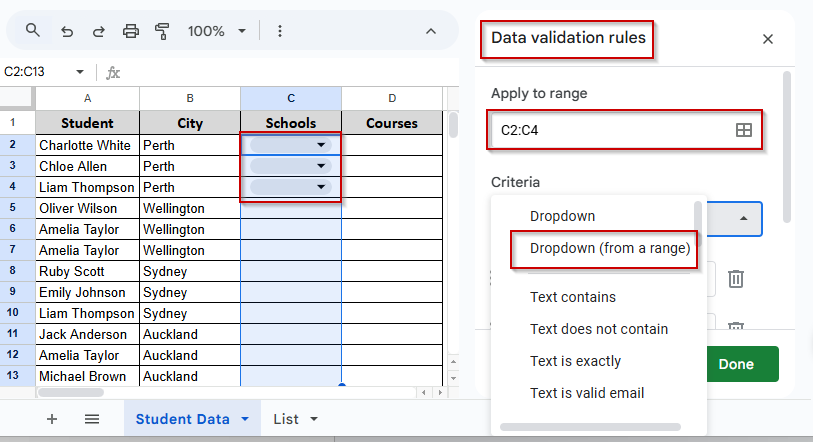
➤ After selecting the Dropdown (from a range), you will see another box appear. Click on the range icon.
➤ You will see a pop-up box arrive. Write Perth inside this box. And Click Ok.
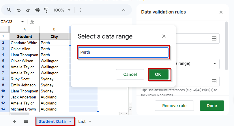
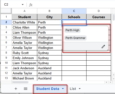
➤ It will call data from the Perth Name Ranges, and you will see the available schools in Perth when you click the drop-down on Column C.
Note:
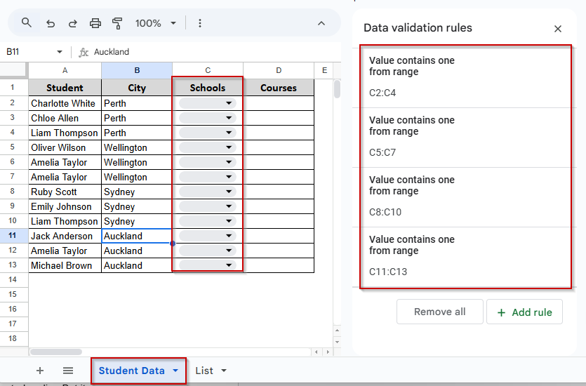
Unfortunately, there is no dynamic method to apply these rules to other cities. Therefore, we have to manually do the same process for other cities.
Follow the same steps for the other cities, and you will see schools from other cities appear under the drop-down menu. After finishing, your data set will look like this:
But this process was not entirely dependent, as we had selected earlier. But it gave you a primary idea. Now let’s create another drop-down list in Column D, which will depend on the school selected in Column C.
To achieve that, we will create a helper column inside our main dataset.
Step 5: Create the Course Drop-down List in the "Student Data" Sheet
We’ll use a formula to fetch the courses based on the selected School.
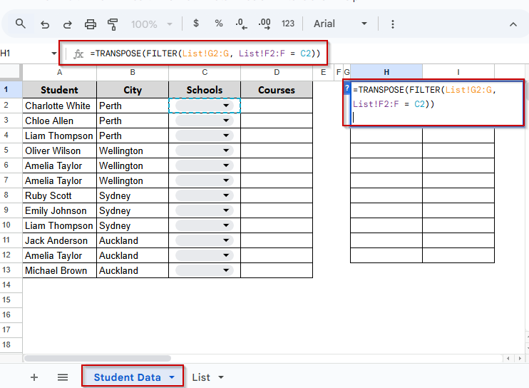
➤ Go to the first cell beside the Courses column. In our case, it’s H2.
➤ Enter this formula:
=TRANSPOSE(FILTER(List!G2:G, List!F2:F = C2))
➤ Press Enter. You’ll see the matching courses appear. Just select the school’s name from the dropdown, and you will see matching courses appear there.
➤ Drag this formula down for the rest of the rows.
➤ Your Student Data Sheet now would look like this:
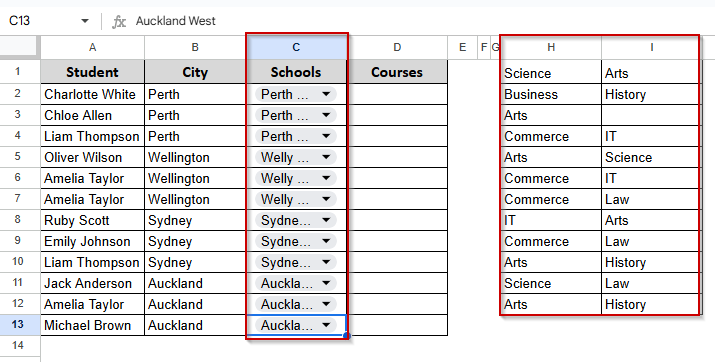
** We created this helper column with some distance just to make the sheet clean. You can create them closer.
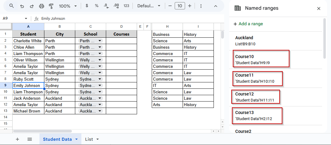
Step 6: Create Named Ranges for Courses
Now we’ll turn each row into a named range.
➤ Go to the Student Data sheet.
➤ Select H1:I1.
➤ From the top menu, click Data → Named ranges.
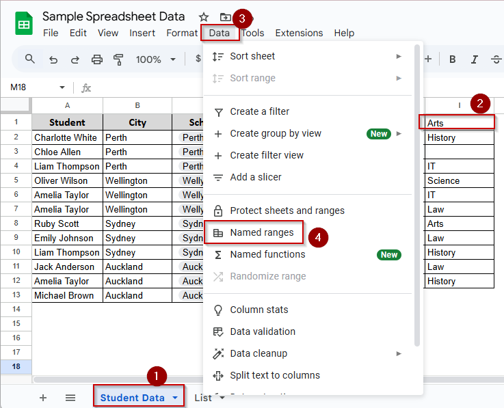
➤ Name this range Course2. Click Done.
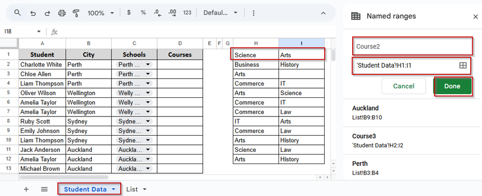
➤ Do the same for the rest:
- Select H2:I2 → Name as Course2
- Select H3:I3 → Name as Course3
…all the way down to Course13.
➤ Finally, your sheet will look like this
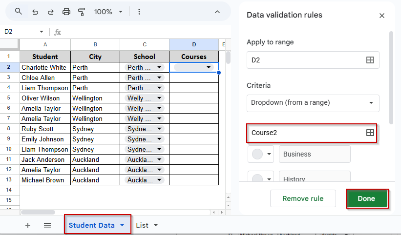
Step 7: Apply Course Drop-Down List in Student Data
Now we’ll create the final dependent drop-down for the Courses column based on the named ranges we just created.
➤ Select D2 .
➤ Click on Data → Data validation.
Your data validation column will appear on the right side of your screen.
➤ Click on Add Rule.
➤ Under Apply to range, enter: D2
➤ Under Criteria, select Dropdown (from a range).
➤ In the range box, type: Course2
➤ Click Done.
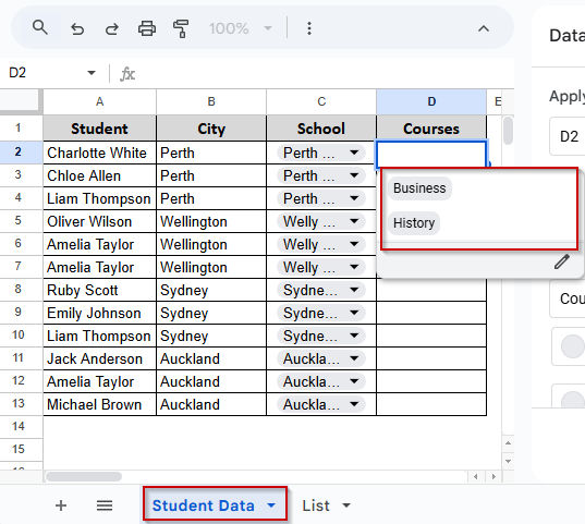
➤ Now let’s try it. Select Perth High from the School Drop Down, and you will see courses listed for this school only. Change it to Perth Grammar, and you will see the courses will change.
➤ Now repeat for each row:
- D3 → Course3
- D4 → Course4
… down to D13 → Course13
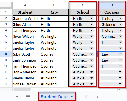
➤ Finally, your sheet will look like this. And you will have a complete multiple-dependent drop-down list in Google Sheets.
Note:
You can safely hide the helper columns after creating the dependent drop-down list. Google Sheets will still recognize the named ranges, and your drop-downs will work smoothly. Just right-click the column letter and choose “Hide column.
Frequently Asked Questions
Can I create more than two levels of dependent dropdowns in Google Sheets?
Sure, you can. You can go three or even four levels deep—like City → School → Course → Subject.
But for more levels, you will need more setups and more helper columns. But the process will be the same.
Can I apply this method inside Google Forms connected to a Sheet?
Unfortunately, Google Forms does not support dynamic or dependent dropdowns. You can use this feature in Google Sheets only.
How can I reset dependent dropdowns when the parent selection changes?
Unfortunately, Google Sheets doesn’t do this automatically. Therefore, you have to use Apps Script to clear the Child cell whenever the parent cell changes. Otherwise, the user will don’t find the accurate selection.
Concluding Words
In this article, you learned how to create a multiple-dependent drop-down list in Google Sheets. Though the process is manual somewhere, after finishing, you will get a dynamic dropdown list.
We have added the worksheet. You can download the worksheet for practice purposes. Also, if you have any specific problems or questions, please ask us in the comment box below.