
Highlighting entire rows in Excel using conditional formatting is the best technique when we work with large datasets. This method helps us to identify specific rows based on defined criteria, and makes data analysis more efficient. This method can bring clarity and focus to our spreadsheets when we manage project timelines, employee lists, or financial records.
To highlight an entire row in Excel with conditional formatting, follow these simple steps:
➤ Select the full data range you want to apply formatting to.
➤ Go to the Home > Conditional Formatting > New Rule.
➤ Choose “Use a formula to determine which cells to format.”
➤ Enter a formula using the row’s identifying condition (e.g., =$B2=”Completed”).
➤ Click Format, choose a fill color, and hit OK to apply.
This article explains how to highlight an entire row in Excel using the Conditional Formatting for Cell Value, Drop Down Selection, Blank, Logical Functions and Numeric Criteria.
Highlight Entire Row in Excel with Conditional Formatting Based on Cell Value
This method highlights the entire row in Excel based on the value of one specific cell in that row. We use this method to visually organize data such as task lists, status reports, or inventory where a specific condition (like “Pending”, “Out of Stock”, “Urgent”, etc.) is meaningful.
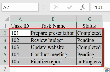
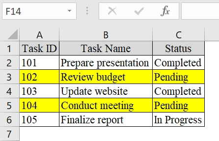
We have an Excel dataset of a task list for a project. The dataset has Task ID in column A, Task Name in column B, and Status in Column C. We will highlight the entire row in Excel of the “Pending” status task using Conditional Formatting with a formula. This will help us visually track which tasks still need to be completed.
Steps:
➤ Click and drag to select your data (e.g., A2:C11 if your table starts from row 2 and has 5 entries and 3 columns).
➤ Go to the Home tab on the Ribbon.
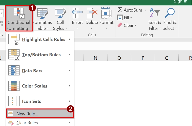
➤ Click on Conditional Formatting. Choose New Rule from the dropdown menu.
➤ In the New Formatting Rule dialog box, select the last option: “Use a formula to determine which cells to format“.

➤ Type the formula into the box: =$C2=”Pending” and click “Format…”.
➥ This formula checks if the value in column C of each row is “Pending“.
➥ The dollar sign before C fixes the column, while the row number updates dynamically.
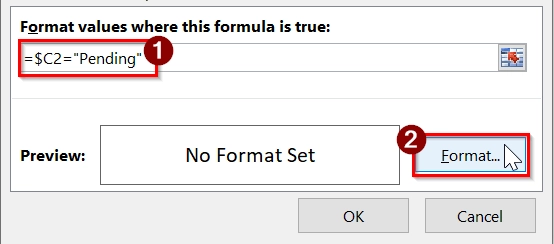
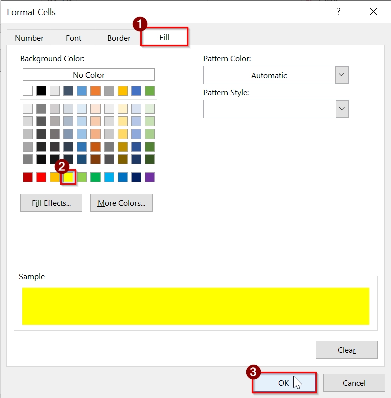
➤ Choose a fill color (like yellow) that will highlight the row. Click OK.
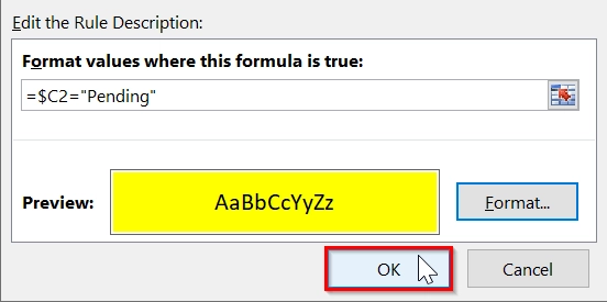
➤ Click OK again to close the dialog.
➤ Your rows where Status is “Pending” will now highlight.
Note:
➥ Make sure the active cell in your selection matches the first row where your data starts.
➥ This method works only if the value is spelled correctly (“Pending” ≠ “pending”).
Highlight Entire Row Based on Numeric Criteria
This method shows how to use Conditional Formatting in Excel to highlight entire rows based on a numeric value, like a performance score or sales target. This is good when we work with datasets and want to visually separate rows that meet specific numeric thresholds.
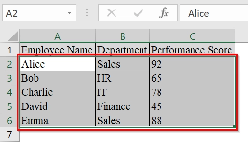
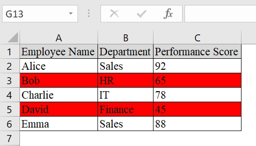
We have a Worksheet that represents a company’s internal performance scorecard. Here, we will identify the underperforming employees using conditional formatting where the “Performance Score” is below 70.
Steps:
➤ Click and drag to select the full range of your data. For example, select cells from A2 to C6.
➤ Go to the Home tab.

➤ In the Styles group, click on Conditional Formatting, then select New Rule.

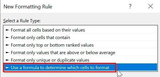
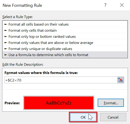
➤ In the dialog box New Formatting Rule, select “Use a formula to determine which cells to format”.
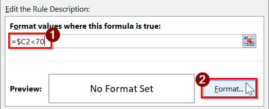
➤ Enter the formula: =$C2<70. Click on the Format… button.
➥ This formula checks if the value in column C (Performance Score) is less than 70 for the current row.
➥ The $C keeps the column fixed, and 2 adjusts for each row.
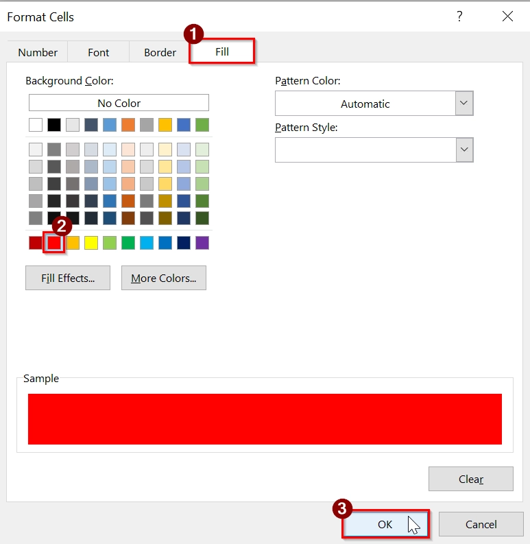
➤ In the Format Cells dialog, choose a Fill color (e.g., light red) and click OK.
➤ Click OK again to exit the New Formatting Rule.
➤ The entire rows where the New Formatting Rule has values less than 70 will now be highlighted.
Note:
➥ Ensure your formula always refers to the first cell in the top-left corner of your selected range.
➥ Avoid applying rules with entire column selections (like A:C) unless necessary; it may slow down performance.
➥ You can use similar logic for greater than (>) or equal to (>=) conditions.
➥ If your data starts in a different row (e.g., row 3), adjust the formula accordingly (e.g., use $C3<70).
Use Logical Functions (AND/OR) to Highlight Entire Row
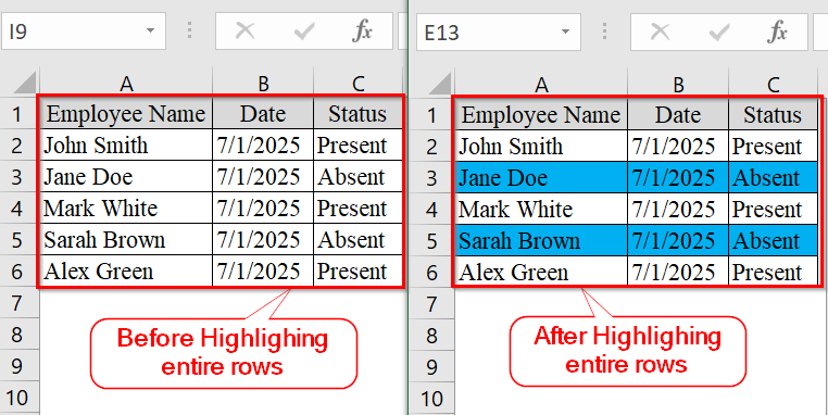
Logical functions like AND and OR can be used in conditional formatting rules to highlight entire rows based on specific cell criteria. This is good when multiple conditions need to be checked (e.g., if a value equals “Absent” or if two columns meet certain values).
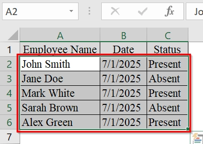
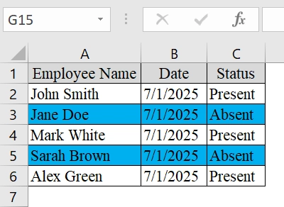
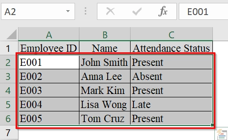
We have a dataset of the HR department to track employee attendance. We will highlight all rows where employees are marked “Absent” to quickly review and act accordingly.
Steps:
➤ Select the entire data range from cell A2 to C6 (assuming headers are in Row 1). This includes all rows and columns that you want to apply formatting to.
➤ Go to the Home tab on the Ribbon.

➤ Click on Conditional Formatting in the Styles group. From the dropdown, select New Rule.

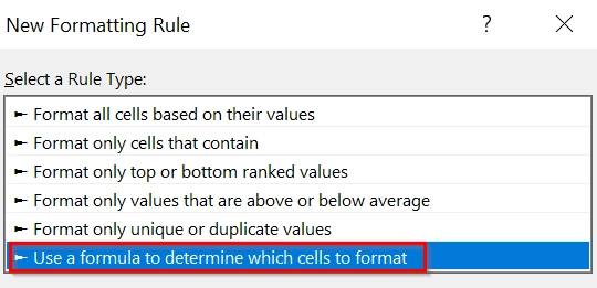
➤ In the dialog box, choose “Use a formula to determine which cells to format”.

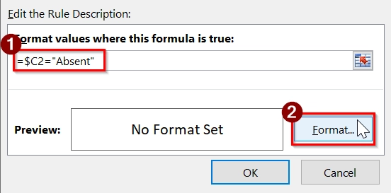
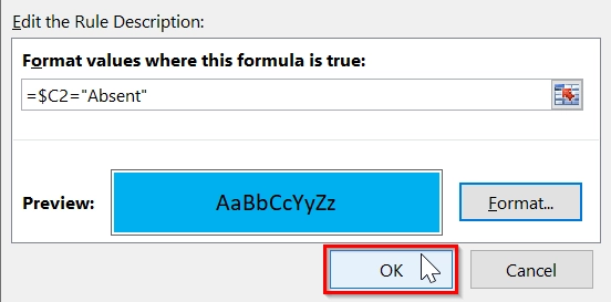
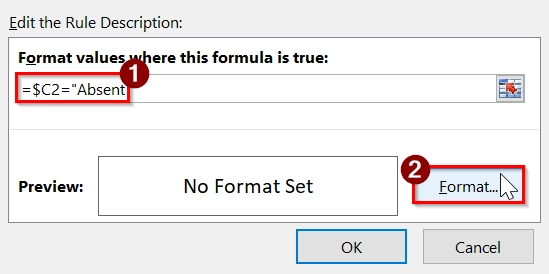
➤ Type the formula in the box. In this case, to highlight rows where the Status is “Absent“, use: =$C2=”Absent”. Then, click the Format… button.
This formula checks if the value in column C for the current row is “Absent“. The $C2 locks the column but allows the row to vary, so it works across all selected rows.
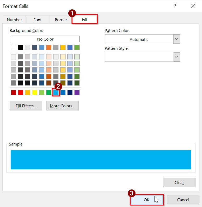
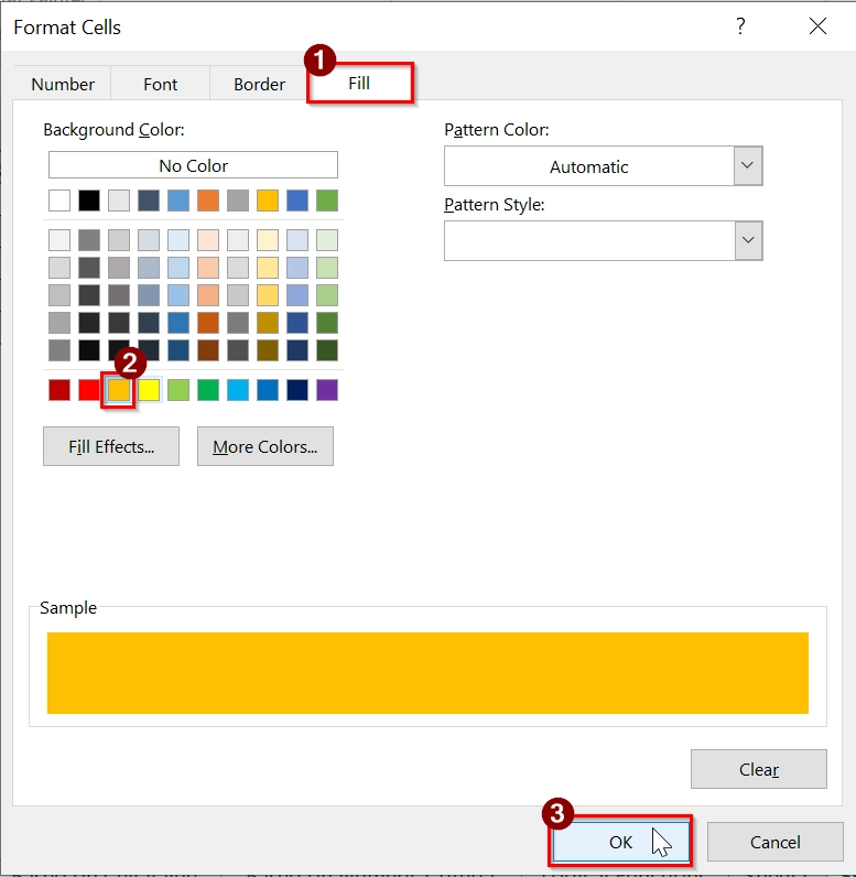
➤ Choose a fill color (e.g., blue) to highlight the row. Click OK.
➤ Click OK on the New Formatting Rule window.
➤ The formatting will now apply to any row where the Status is “Absent“.
Note:
➥ Make sure you start the selection from the top-left data cell (A2 here) and write the formula relative to that row.
➥ Do not include the header row in the selection, unless you want it formatted too.
➥ Excel auto-adjusts formulas for each row within the range.
Highlight Entire Row in Excel Where Any Cell Is Blank
We can highlight the entire row in Excel when any cell in that row is blank. This is good when we want to identify incomplete entries in tables like task sheets, inventory lists, or student records. We use this when we need to visually track rows with missing data across a dataset.
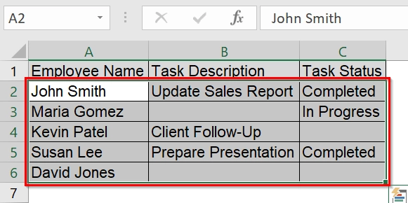
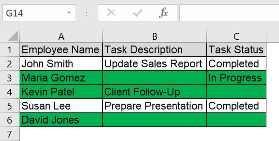
We have an Excel dataset that contains a task tracking sheet. Here, we will identify incomplete rows by highlighting the entire row if the row contains a blank cell.
Steps:
➤ Select the data range. For example, if your table data is from A2 to C6, select the range A2:C6.
➤ Go to Conditional Formatting > New Rule.

➤ In the New Formatting Rule window, choose the last option: “Use a formula to determine which cells to format“.

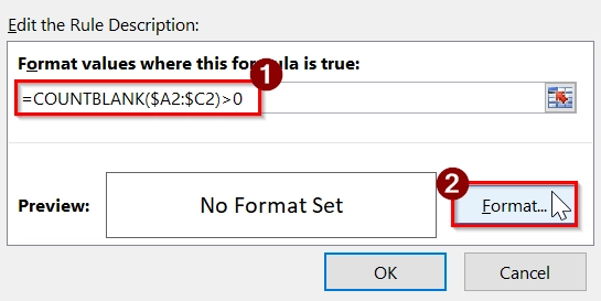
➤ Enter this formula in the box:
=COUNTBLANK($A2:$C2)>0. Click “Format…”.
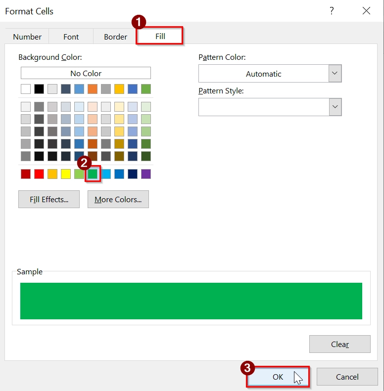
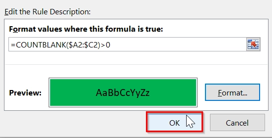
➤ Choose a fill color (e.g., green) to highlight the row. Click OK.
➤ Click OK again to close the rule editor and apply the formatting to your selected range.
➤ The rows in which any cell is blank, will be highlighted.
Highlight Entire Row Based on Cell Value Using Multiple Rules
This method highlights entire rows in a worksheet based on the value in a specific column. This is best when we want to visually differentiate rows where a key condition is met. This method is suitable for quick identification and better data interpretation.
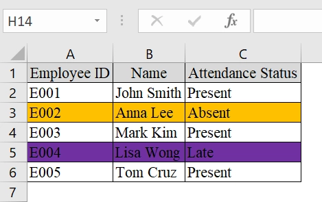
We have a table containing employee attendance status. In this table, we want to highlight the entire row in red if an employee is marked “Absent“, in yellow if marked “Late“, and no highlight if marked “Present“.
Steps:
➤ Select the entire data range you want to apply conditional formatting to (including headers if needed). Example: Select A2:C6 for the sample attendance table.
➤ Click on Conditional Formatting → New Rule.

➤ In the “New Formatting Rule” window, choose “Use a formula to determine which cells to format.”
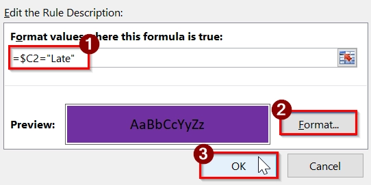
➤ Enter the formula in the formula box: =$C2=”Absent”. Click “Format…”.
➤ Go to the Fill tab, and choose an orange fill color. Press OK.
➤ Repeat Steps 2 to 5 with the formula: =$C2=”Late”. Choose a purple fill color this time. Click OK.
➤ The entire rows will now be highlighted based on the “Attendance Status”.
Note:
You can add more rules for different statuses or criteria using similar steps.
Highlight Entire Row If Matches with Drop Down Selection
To highlight an entire row in Excel when a specific drop-down option is selected in a particular column we can use this process. This is also used for managing task lists, project trackers, or workflow sheets to visually flag rows to meet a specific status or condition. This is best for datasets that use drop-down menus for data consistency.
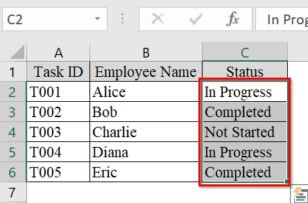
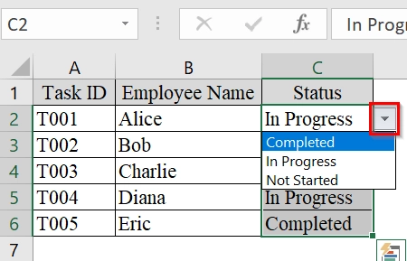
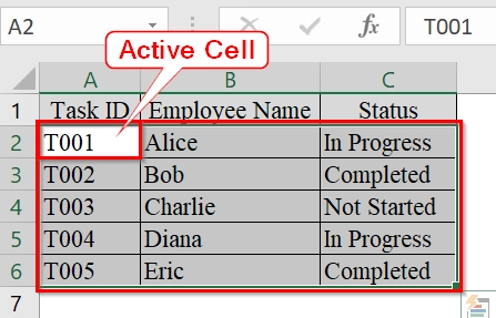
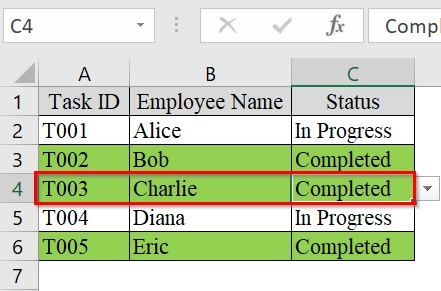
We have an Excel worksheet that tracks the status of tasks assigned to different employees. We will highlight the row that tasks are “Completed” using drop-down selection in the “Status” column.
Steps:
➤ Select the cells in Column C where you want to include the drop-down (e.g., C2:C6).
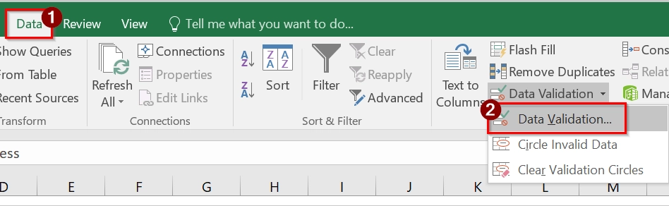
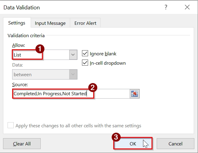
➤ Go to the Data tab → Click Data Validation.
➤ Under Allow, choose List → In the Source box, type: Completed,In Progress,Not Started. Click OK.
➤ This will add a drop-down to each selected cell.
➤ Select the Entire Data Range for Formatting range A2:C6 (or as per your dataset size). Make sure the active cell is A2 when you start the conditional formatting.
➤ Go to the Home tab.

➤ Open Conditional Formatting Rules. Choose “New Rule”.

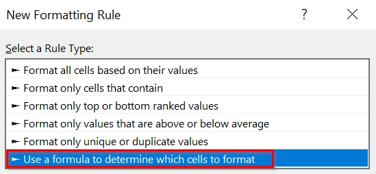
➤ In the New Formatting Rule window, select the option “Use a formula to determine which cells to format”.
➤ In the formula field, type this: =$C2=”Completed”. Click the Format button.
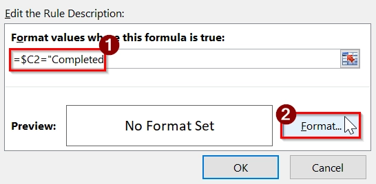
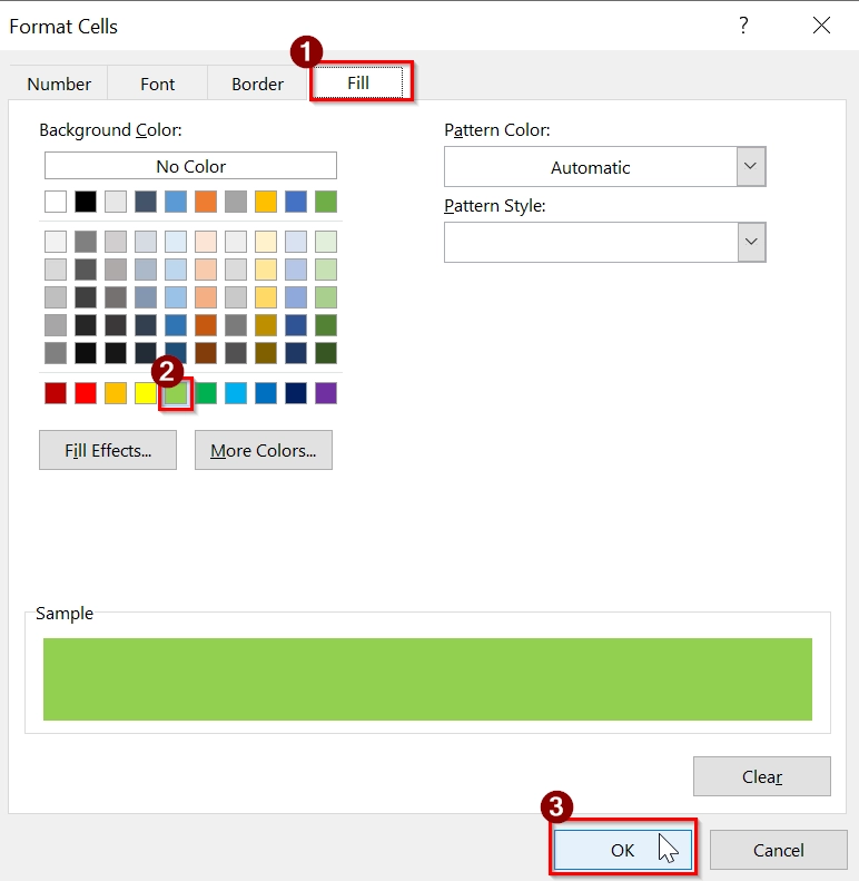
➤ Choose a Fill color (e.g., light green) → Click OK.
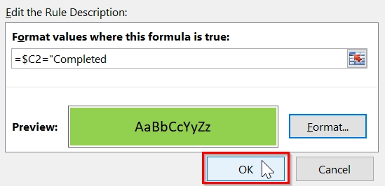
➤ Click OK again to apply the rule.
➤ The rows with status “Completed” will be highlighted.
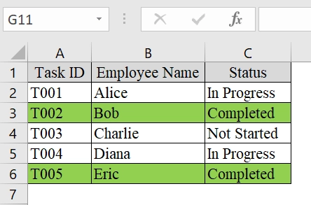
➤ Now, when you select “Completed” from the drop-down in column C, the entire row from Columns A to C will be highlighted with the chosen color.
Note:
➥ Make sure the formula references the column with the drop-down ($C2) and uses an absolute column reference ($C) to apply correctly across the row.
➥ You must select the entire range before applying the rule so that full rows get highlighted, not just single cells.
Frequently Asked Questions
Can I highlight multiple rows based on different conditions?
Yes, you can create multiple conditional formatting rules with different formulas targeting different criteria.
Will the formatting update automatically if the data changes?
Absolutely. Conditional formatting in Excel is dynamic, it updates as soon as the underlying data meets or no longer meets the condition.
How can I remove the formatting later?
Select the range, go to Home > Conditional Formatting > Clear Rules, and choose either from the selected cells or the entire sheet.
Can this be applied to tables with filters?
Yes. Conditional formatting works with filtered data and will apply formatting even as filters are added or removed.
Concluding Words
Highlighting an entire row in Excel using Conditional Formatting with a formula is a powerful and simple method to improve data visualization. By this technique, we can make spreadsheets more informative and easier to interpret without manually adjusting cell styles.