Sometimes in Excel, you need to match a date to a specific range instead of looking for an exact match. For instance, when tracking sales across multiple promotions, you might want to label each order based on the period it was placed in.
This is where VLOOKUP with date ranges becomes useful. VLOOKUP usually matches exact values, but it can also return results based on ranges when the setup is correct. You can use it to pull pricing tiers, seasonal labels, or promotional periods based on the date of each transaction.
In this article, we’ll learn how to use VLOOKUP to match dates to defined ranges using a simple lookup table.
Here’s how to use Excel VLOOKUP with a date range:
➤ Open your dataset in Excel.
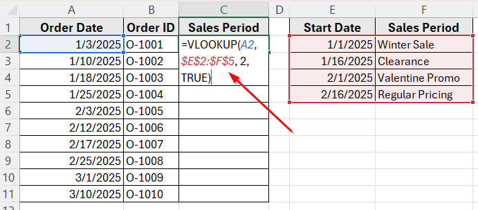
➤ Click on cell C2, where we want to display the sales period for the first order.
➤ Enter the following formula
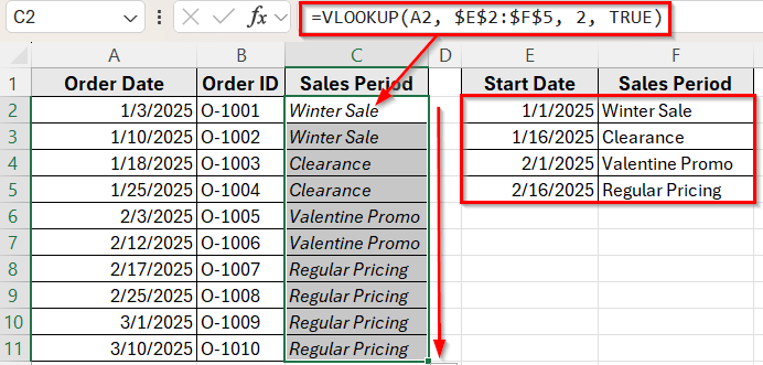
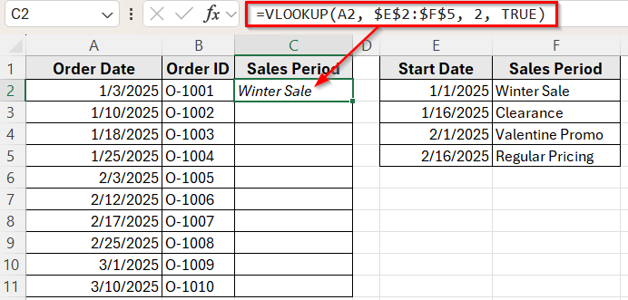
=VLOOKUP(A2, $E$2:$F$5, 2, TRUE)
➤ Press Enter, and you’ll see the sales period appear based on the order date.
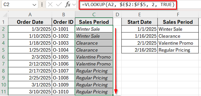
➤ Now, drag the fill handle down to copy the formula to the rest of the rows.
Using VLOOKUP Function with Approximate Match to Return a Value by Date Range
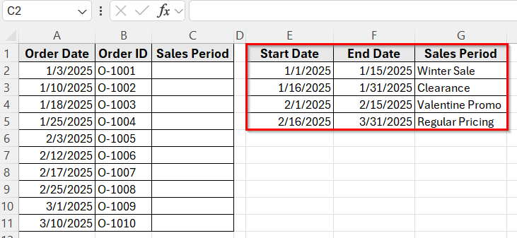
In the following dataset, we have a simple order log that records customer purchases and their dates. Column A lists the Order Dates, Column B contains the Order IDs, and Column C will display the Sales Period based on the order date.
On the right, we’ve created a lookup table that defines the Start Date of each sales period in Column E and the corresponding Sales Period Name in Column F. Our goal is to return the correct sales period for each order depending on when it was placed.
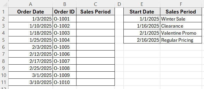
We’ll use this dataset to demonstrate how to use VLOOKUP to match a date to its correct range and return the appropriate value in Excel.
The VLOOKUP function is one of the simplest ways to assign a value based on a date range. This method works by using a lookup table that contains the start dates of each range. When you use VLOOKUP in approximate match mode, Excel will return the value that matches the latest date less than or equal to the lookup date.
Here’s how to apply this method:
➤ Open your dataset in Excel.
➤ Click on cell C2, where we want to display the sales period for the first order.
➤ Enter the following formula
=VLOOKUP(A2, $E$2:$F$5, 2, TRUE)
➤ Press Enter, and you’ll see the sales period appear based on the order date.
➤ Now, drag the fill handle down to copy the formula to the rest of the rows.
Combining INDEX and MATCH Functions to Check If a Date Falls Between Two Columns
The combination of INDEX and MATCH is a great option when you want to return a value based on a date that falls within a specific range. This method works well when each period has a clear start date and end date listed in your lookup table. It gives you full control and works accurately even when the ranges are uneven.
First, update your lookup table so it includes both Start dates and End dates.
Here’s how to apply this method:
➤ Click on cell C2, where we want to return the sales period name.
➤ Enter the following formula:
=INDEX($G$2:$G$5, MATCH(1, (A2 >= $E$2:$E$5) * (A2 <= $F$2:$F$5), 0))
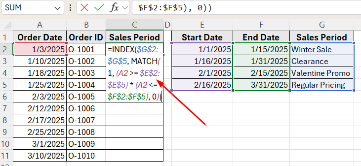
➤ Press Ctrl + Shift + Enter if you are using Excel 2016 or an earlier version. In Excel 365 or Excel 2019, just press Enter .
➤ Now you’ll see the sales period appear based on the order date.
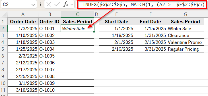
➤ Next, drag the fill handle down to apply the formula to the rest of the rows.

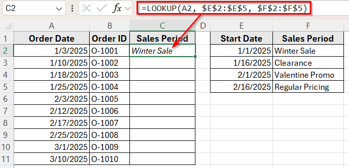
Use LOOKUP Function for Sorted Date Ranges
The LOOKUP function is another quick way to return a value based on a date range. It works well when your data is sorted in ascending order. LOOKUP scans the range and finds the largest value that is less than or equal to the lookup date.
This method is simple and effective when your date ranges start on fixed days, and you only need a one-way check using the start dates.
Here’s how to use it:
➤ Click on cell C2, where you want to show the sales period.
➤ Enter the following formula:
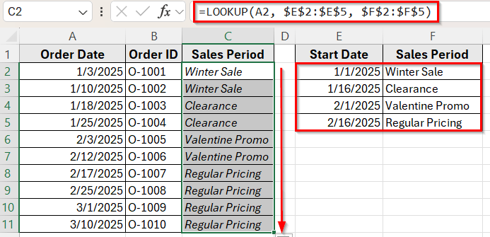
=LOOKUP(A2, $E$2:$E$5, $F$2:$F$5)
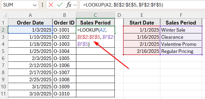
➤ Press Enter. LOOKUP function returns the value in column F that matches the latest date less than or equal to the value in A2.
➤ Then, drag the fill handle down to apply the formula to the other rows.
Frequently Asked Questions
How do I use VLOOKUP in Excel for a date range?
You can use VLOOKUP with a helper column or use alternative functions like LOOKUP, INDEX with MATCH, or nested IFs. These methods help return values when the lookup date falls within a start and end date range.
Does VLOOKUP work with date ranges directly?
VLOOKUP doesn’t support date ranges on its own. It looks for exact matches or the nearest value less than or equal to the lookup value. To check full ranges with both start and end dates, use a formula that combines INDEX and MATCH.
How do you do a VLOOKUP if a cell contains a date?
If a cell contains a date, you can use VLOOKUP just like you would with numbers or text. Make sure the lookup column also contains actual Excel date values, not text. Then use:
=VLOOKUP(A2, LookupRange, ColumnNumber, TRUE)
Use the TRUE argument to find the closest date that is less than or equal to the lookup value, assuming the data is sorted by date.
Wrapping Up
Looking up values by date range in Excel is easier once you know which formula fits your task. VLOOKUP works well for basic start-date checks. LOOKUP provides a quick alternative when the list is sorted. For more control, the combination of INDEX and MATCH can check full date ranges with start and end limits.
Each method serves a specific purpose depending on how your data is organized. With the right setup, you can quickly return relevant values for reports, sales periods, timelines, and more.