

When planning finances or solving business problems, you often need to find the exact input that leads to a desired result. That’s where Goal Seek in Excel becomes useful. It allows you to work backward by setting a target value and letting Excel calculate the input needed to reach that goal. In this tutorial, we will walk you through how to use Goal Seek in Excel with three examples.
To use Goal Seek in Excel:
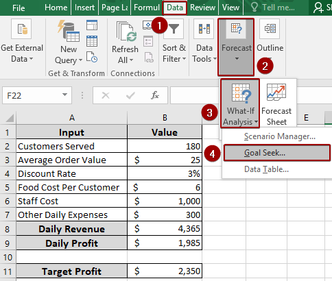
➤ Go to the Data tab, click What-If Analysis, and choose Goal Seek.
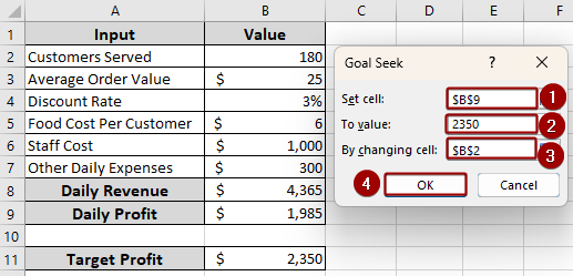
➤ In the Goal Seek dialog box, choose the cell containing the formula (like Daily Profit) in the Set cell field.
➤ Enter the target value you want (e.g., $2,350).
➤ Choose the input cell you want to change (like Customers Served) in the By changing cell field.
➤ Click OK, and Excel will calculate the required customer to achieve the specified target.
What Is Goal Seek in Excel and How Does It Work?
Goal Seek is a built-in what-if analysis tool that finds the input value needed to reach a specific output. Instead of manually guessing different inputs, Goal Seek allows you to work backward from a desired result. You define the goal (target value), and Excel automatically adjusts one input cell until the formula returns that exact result.
The following are the steps on how Goal Seek works in Excel:
- Start with a formula: First, make sure you have a formula in your sheet, something that calculates a result based on an input, like total sales.
- Decide your goal: Next, put your desired result you want. For example, maybe you want your target profit to be exactly $500.
- Pick the input to change: Choose which cell Excel should change to reach your goal, like adjusting the customer served or number of items sold.
- Let Excel do the work: Finally, run Goal Seek, and Excel will automatically test different values until the formula gives you the result you wanted.
3 Examples to Use Goal Seek in Excel
In this guide, we will show you how to use Goal Seek through three real-life examples: determining number of customers to get target profit, calculating time to reach target production, and finding the minimum score needed on a final exam.
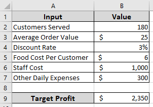
Suppose we have a dataset containing Customers Served, Average Order Value, Discount Rate, Food Cost Per Customer, Staff Cost, Other Daily Expenses, and Target Profit as inputs. Now, we will calculate the Daily Profit and use Goal Seek to find the exact customer needed to meet the target profit.
Example 1: Determining Number of Customers to Get Target Profit
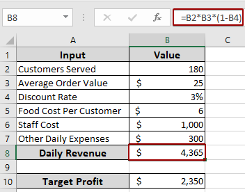
First, we will calculate the Daily Revenue.
➤ Choose cell B8 and input the formula below.
=B2*B3*(1-B4)
This formula calculates the Daily Revenue by multiplying the Customers Served by the Average Order Value and subtracting the Discount Rate.
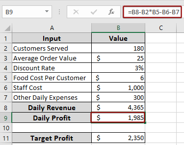
Next, we will calculate the Daily Profit.
➤ Choose cell B9 and input the formula below.
=B8-B2*B5-B6-B7
This formula calculates the Daily Profit by subtracting the Food Cost, Staff Cost, and Other Daily Expenses from the Daily Revenue.
To apply Goal Seek and determine the number of customers required to achieve the target profit:
➤ Click on the Data tab from the menu bar.
➤ In the Forecast group, click What-If Analysis.
➤ From the drop-down menu, choose Goal Seek.
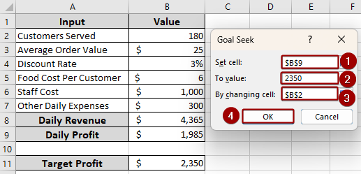
In the Goal Seek dialog box, you will define your target and the cell that Goal Seek should change to reach that target.
➤ In the Set cell field, enter B9, as this is the cell containing the formula for our Daily Profit.
➤ In the To value field, enter 2350, which is our desired target profit.
➤ In the By changing cell field, enter B2, as we want to find the number of Customers Served required to achieve the target profit.
➤ Finally, click OK.
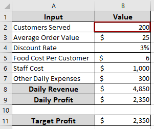
This way, the Customers Served value in cell B2 will change to 200, indicating that the restaurant needs to serve 200 customers to achieve a target profit of $2,350.
Example 2: Calculating Time to Reach Target Production
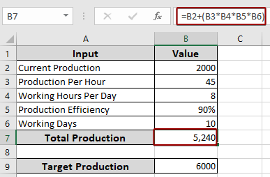
Goal Seek can also be used to determine the amount of time required to achieve a specific production target. Imagine a dataset containing Current Production, Production Per Hour, Working Hours Per Day, Production Efficiency, and Working Days. Here, we will calculate the Total Production and use Goal Seek to find out the number of Working Days needed to achieve a target production of 6,000 units.
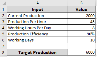
First, we will calculate the Total Production.
➤ Select cell B7, and write the following formula.
=B2+(B3*B4*B5*B6)
This formula calculates the Total Production by adding the Current Production to the production achieved during the specified Working Days, considering the Production Per Hour, Working Hours Per Day, and Production Efficiency.
To start the Goal Seek process and find the required number of working days:
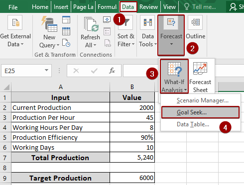
➤ Click on the Data > Forecast > What-If Analysis > Goal Seek.
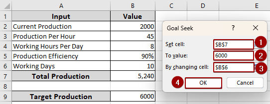
In the Goal Seek dialog box, you will define your target production and the cell that Goal Seek should adjust to achieve that target.
➤ In the Set cell field, enter B7, as this cell contains the formula for our Total Production.
➤ In the To value field, enter 6000, which is our desired production target.
➤ In the By changing cell field, enter B6, as we want to find the number of Working Days required to achieve the target production.
➤ Finally, click OK.
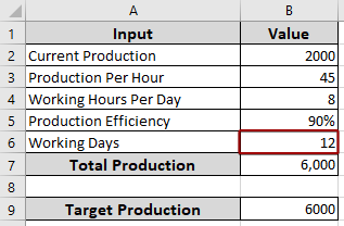
As a result, the Working Days value in cell B6 will change to approximately 12, indicating that it will take approximately 12 working days to reach a Total Production of 6,000 units.
Example 3: Computing Minimum Number for Final Exam
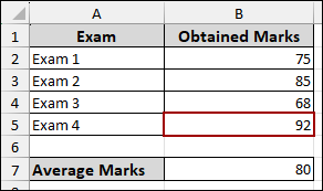
In this example, we will determine what score is needed in one particular exam to reach a desired overall average. Suppose we have a dataset containing four exams and their obtained marks. In Exam 4, the marks cell is blank, as we will use Goal Seek to find out the score for Exam 4 needed to achieve a Total Marks (average) of 80.
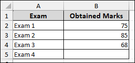
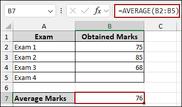
First, we will calculate the average of all marks using the AVERAGE function.
➤ Choose cell B7, and put the formula in the cell.
=AVERAGE(B2:B5)
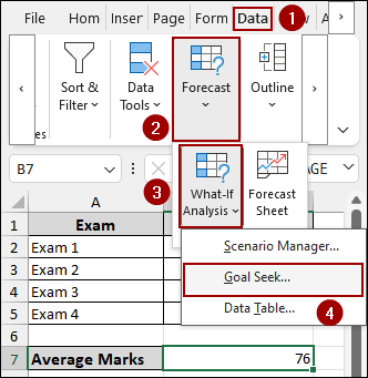
To begin the Goal Seek process and find the required exam score:
➤ Click on the Data > Forecast > What-If Analysis > Goal Seek.
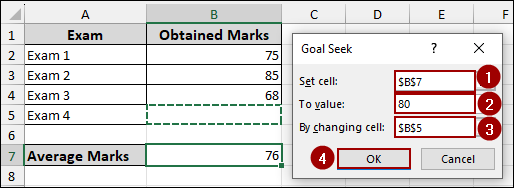
In the Goal Seek dialog box, you will specify your target average and the cell that Goal Seek should modify to reach that target.
➤ In the Set cell field, enter B7, as this cell contains the formula for our Total Marks (average).
➤ In the To value field, enter 80, which is our desired average score.
➤ In the By changing cell field, enter B5, as we want to find the score for Exam 4 that achieves the desired average.
➤ Finally, click OK.
As a result, the score for Exam 4 in cell B5 will change to 92, indicating that you need to score 92 in Exam 4 to achieve an overall average of 80.
Downloadable Resources
Get our practice workbook or necessary files that we have worked with to prepare this article.
Examples with Goal Seek in Excel.xlsx
Frequently Asked Questions
How can I get more precise results using Goal Seek?
By default, Goal Seek uses Excel’s standard calculation precision. To improve accuracy, go to File > Options > Formulas. Under Calculation options, reduce the Maximum Change value (e.g., 0.0000001). This ensures Excel iterates with greater precision when running Goal Seek.
Why is Goal Seek not working in my Excel sheet?
There are two common reasons. First one is, you need to set the cell that contain a valid formula. If it’s a static number, Goal Seek won’t work. The second one is a circular reference (when a formula refers back to itself) that can block Goal Seek. Check for and remove any circular references.
Why does Goal Seek give a negative number sometimes?
If you are using financial functions like PMT, Excel shows cash outflows as negative. The result is still correct, just interpret the negative sign as a payment.
Concluding Words
Above, we have explored how to use Goal Seek in Excel to work backward from a desired outcome and find the exact input needed. This feature is especially useful in scenarios like loan planning, profit targeting, or grade forecasting. If you have any questions, feel free to leave them in the comments below.