

When planning or analyzing data in Excel, it’s crucial to understand how changes in your inputs can affect the outcome. Excel offers powerful what-if analysis tools like Scenario Manager, Goal Seek, and Data Tables that let you explore different possibilities without altering your original data. In this article, we will teach you each technique step by step so you can confidently model, forecast, and plan in Excel.
To use what-if analysis with Goal Seek in Excel, follow the steps below.
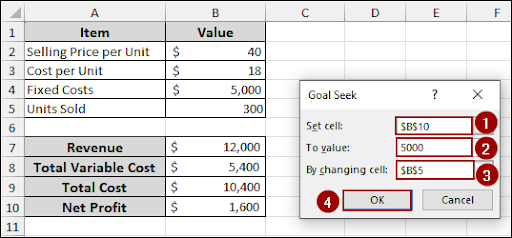
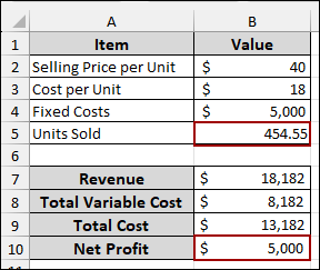
➤ Go to the Data tab, click What-If Analysis, and choose Goal Seek.
➤ In the Goal Seek dialog box:
For “Set cell“, select the cell that contains your target outcome, which is B10 (Net Profit).
For “To value“, enter your desired net profit, which is 5000.
For “By changing cell“, select the input cell that Goal Seek should adjust to reach your target.
➤ Press OK, and Excel will automatically change the input(cell B5) to reach your goal with net profit of $5,000(cell B10).
What Is a What-If Analysis in Excel?
What-if analysis in Excel lets you explore how changes in inputs affect your final results. Instead of manually changing different values, Excel offers built-in tools that automate the process and help you evaluate various scenarios. There are three main types of what-if analysis:
Scenario Manager: It lets you store and switch between multiple sets of input values to compare different outcomes.
Goal Seek: This helps you find the exact input needed to reach a specific result.
Data Tables: It allows you to test how one or two variables affect your results across a range of values.
Using Scenario Manager for What-if Analysis in Excel
Using Scenario Manager for what-if analysis in Excel helps you compare different sets of inputs and their outcomes. Instead of manually changing values one by one, you can store multiple scenarios in one place. This makes it easy to switch between best-case, worst-case, or custom cases. In this section, we’ll show you how to set up and use Scenario Manager for different scenarios.
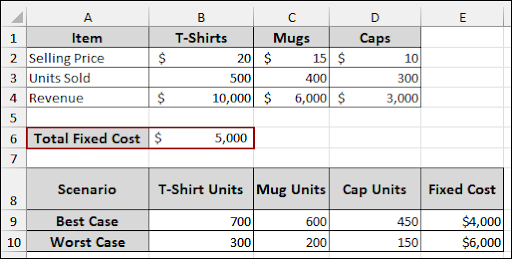
Suppose we have a sample dataset containing Selling Price and Units sold for 3 items: T-shirts, Mugs, and Caps. In addition, we have 2 types of scenarios: Best case and Worst case. The best case scenario consists of higher units sold with low fixed costs. Similarly, the worst case has lower units sold and higher fixed costs. Now, we will demonstrate both scenarios using the Scenario Manager for what-if analysis in Excel.
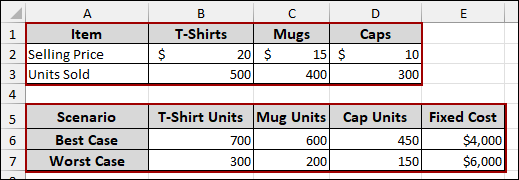
First, we will calculate the “Revenue” for each item.
➤ Select cell B4, and put the following formula and hit ENTER.
=B2*B3
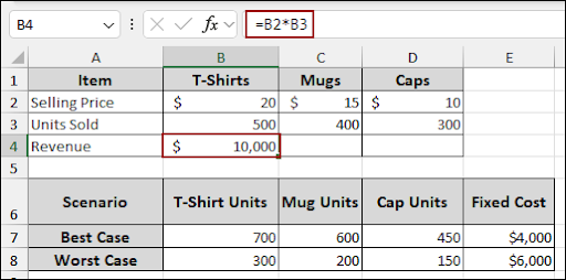
➤ Drag the fill handle to the right to apply this formula to calculate the revenue for “Mugs” and “Caps” as well.
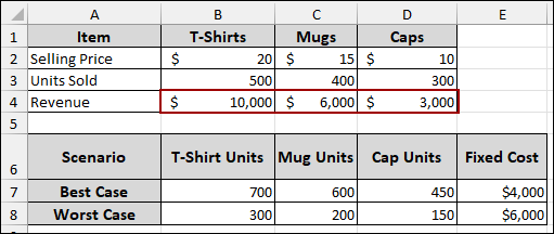
➤ Now, input your “Total Fixed Cost”.
Here, we have put a Total Fixed cost of 5,000 in cell B6.
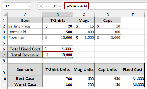
➤ To calculate the “Total Revenue,” select cell B7 and input the formula below.
=B4+C4+D4
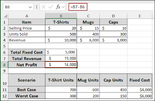
➤ Finally, to determine the “Net Profit,” select the cell and type the formula below.
=B7-B6
Thus, we have successfully created a basic financial model, providing a clear overview of our revenue, costs, and profit. Now, we will analyze both our scenarios’ best and worst cases.
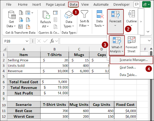
➤ First, navigate to the Data tab in the Excel ribbon.
➤ In the Forecast group, click on What-If Analysis.
➤ From the drop-down menu, select Scenario Manager.
This will open the Scenario Manager dialog box.
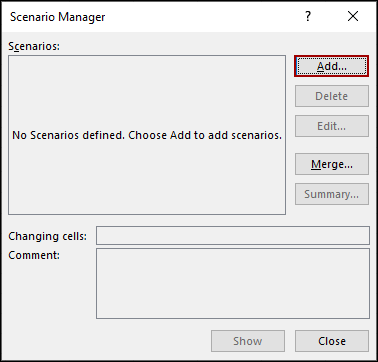
➤ In the Scenario Manager dialog box, click on the Add button.
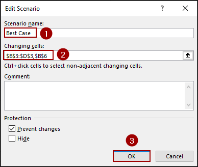
➤ In the Scenario name section, name your scenario as Best Case.
➤ For “Changing cells“, select the cells that will vary in your scenario.
In our model, these are the varying cells “Units Sold” for T-Shirts, Mugs, and Caps ($B$3:$D$3) and the “Total Fixed Cost” ($B$6). You can select multiple, non-adjacent cells by holding down the Ctrl key while clicking.
➤ Click OK.
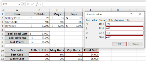
➤ In the Scenario Values dialog box, enter the specific values for your “Best Case” scenario:
For T-Shirt Units ($B$3), enter 700.
For Mug Units ($C$3), enter 600.
For Cap Units ($D$3), enter 450.
For Fixed Cost ($B$6), enter 4000.
➤ Hence, click OK.
➤ Similarly, insert the specific values for your “Worst Case” scenario:
For T-Shirt Units ($B$3), enter 300.
For Mug Units ($C$3), enter 200.
For Cap Units ($D$3), enter 150.
For Fixed Cost ($B$6), enter 6000.
➤ Finish the process by hitting OK.
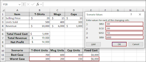
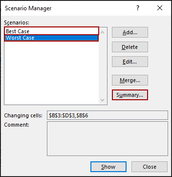
➤ Thus, both “Best Case” and “Worst Case” scenarios are added.
➤ Now, click on the Summary button.
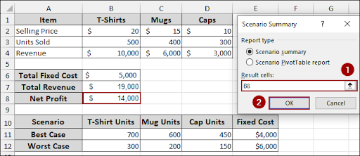
➤ Hence, for “Result cells“, specify the cell that contains the final outcome you want to analyze across scenarios.
➤ Click OK.
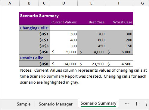
Finally, Excel will generate a new worksheet titled “Scenario Summary”, which presents a comprehensive report. This summary outlines how your changing cells affect the “Net Profit” under the best and worst scenarios.
Applying Goal Seek for What-if Analysis
Goal Seek in Excel is a powerful tool for testing how changing one input can achieve a specific outcome. Instead of guessing values manually, Goal Seek automates the process. It’s especially useful when you are targeting a specific output. Goal Seek is designed to adjust a single input cell; it cannot work with multiple cells at once. In this section, we’ll show you how to use Goal Seek with a simple example.
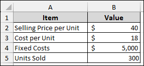
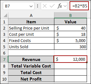
Suppose we have a dataset with the following items and their initial values: Selling Price per Unit: $40 (in cell B2), Cost per Unit: $18 (in cell B3), Fixed Costs: $5,000 (in cell B4), Units Sold: 300 (in cell B5). Now, we will set up formulas to calculate our financial metrics and then use Goal Seek to reach a target value.
➤ To calculate Revenue, select cell B7.
➤ In the formula bar, input the formula (Selling Price per Unit * Units Sold) and press ENTER.
=B2*B5
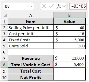
➤ Now, calculate Total Variable Cost, select cell B8.
➤ In the formula bar, insert the formula (Cost per Unit * Units Sold) and press ENTER.
=B3*B5
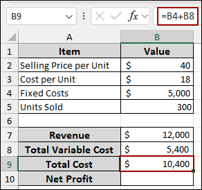
➤ Then, compute Total Cost, select cell B9.
➤ In the formula bar, put the formula (Fixed Costs + Total Variable Cost) and press ENTER.
=B4+B8
➤ Finally, to calculate Net Profit, select cell B10.
➤ In the formula bar, input the formula (Revenue – Total Cost) and press ENTER.
=B7-B9
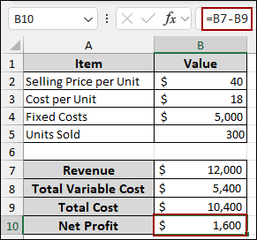
Now our financial model is set up, let’s use Goal Seek to find out how many units we need to sell to achieve a specific net profit, for example, $5,000.
➤ Navigate to the Data tab in the Excel ribbon.
➤ In the Forecast group, click on What-If Analysis.
➤ From the drop-down menu, select Goal Seek.
This will open the Goal Seek dialog box.
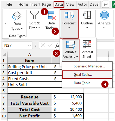
➤ In the Goal Seek dialog box:
For “Set cell“, select the cell that contains your target outcome, which is B10 (Net Profit).
For “To value“, enter your desired net profit, which is 5000.
For “By changing cell“, select the input cell that Goal Seek should adjust to reach your target.
➤ Click OK.
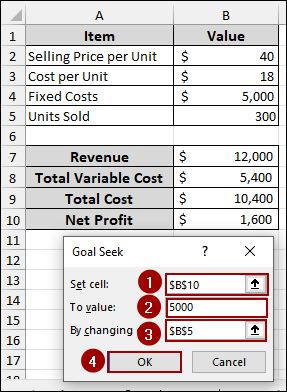
Thus, Excel will automatically adjust the “Units Sold” to the required number to achieve your desired “Net Profit,” providing an instant solution to your what-if scenario.
Using Data Tables for What-if Analysis in Excel
Data Tables in Excel help you test how changing one or two inputs affects the outcome of a formula. Instead of updating values manually, you can automate the process across a range of possibilities. This makes it easy to compare results side by side. In this section, we’ll show you how to use one-variable, two-variable, and three-variable data tables for quick analysis.
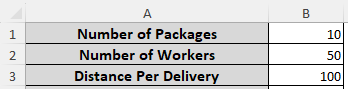
Let’s assume we have a dataset with the following inputs: Number of Packages (B1), Number of Workers (B2), and Distance Per Delivery (B3).
One Variable Sensitivity Analysis
One Variable sensitivity analysis shows how changes in a single input affect the result of a formula. In this section, we will show you how to set it up using Excel’s Data Table feature.
First, we will calculate the Average Delivery Time in Minutes.
➤ Select cell B4, input the formula below, and press Enter.
=(B1*B3)/B2
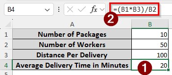
➤ Now, we will create the structure for the data table.
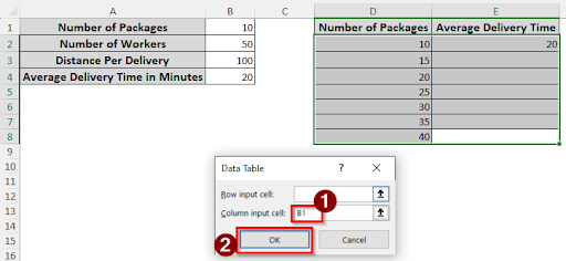
➤ In cell D1, enter “Number of Packages” and in cell E1, enter “Average Delivery Time”.
➤ Below “Number of Packages,” list various numbers of packages that can be in a delivery company, for example, from 10 to 40 in column D (cells D2:D8).
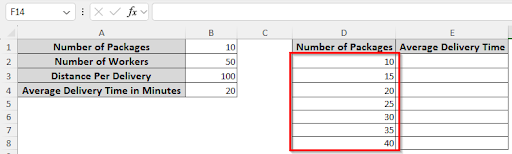
➤ Write down the formula in cell E2 and hit ENTER.
=B4
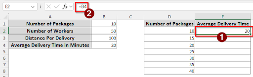
➤ Select the entire range of your data table (cells D2 to E8).
➤ Navigate to the Data tab in the Excel ribbon.
➤ In the Forecast group, click on What-If Analysis.
➤ From the drop-down menu, select Data Table.
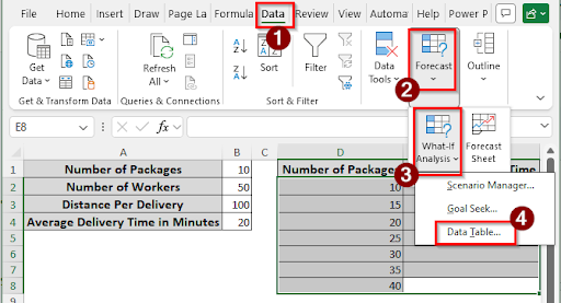
➤ In the Data Table dialog box:
Leave “Row input cell” blank, as our varying input is in a column.
For “Column input cell“, select the cell that holds your original number of packages, which is B1. This tells Excel to substitute the values from column D into cell B1 to calculate the delivery time.
➤ Click OK.
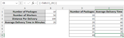
Finally, your data table will populate, showing you the calculated “average delivery time” for each “number of packages” that was specified.
Two Variable Sensitivity Analysis
Sometimes, you need to analyze how two different input variables affect a formula’s outcome. A two-variable Data Table is perfect for this, as it presents a grid showing the results for all combinations of your two changing inputs. Below are the steps for performing a what-if analysis using a two-variable Data Table.
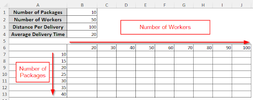
Suppose we have the same delivery time calculation model set up as before. Here, let’s create the layout for our two-variable data table. Along the top row, starting from cell B6 and moving rightward, list the different “Number of Workers” we want to analyze. Down the first column, starting from cell A7 and moving downward, list the various “Number of Packages” we want to analyze.
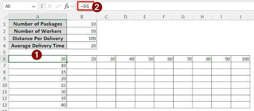
➤ In cell A6, enter the formula below.
=B4
➤ Select cells B6 to J13, containing the whole table.
➤ Navigate to the Data tab in the Excel ribbon.
➤ In the Forecast group, click on What-If Analysis.
➤ From the drop-down menu, select Data Table.
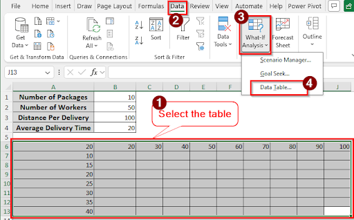
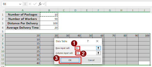
➤ In the Data Table dialog box:
For “Row input cell“, select the cell that holds the number of workers, which is B2.
For “Column input cell“, select the cell that holds the number of packages, which is B1.
➤ Click OK.
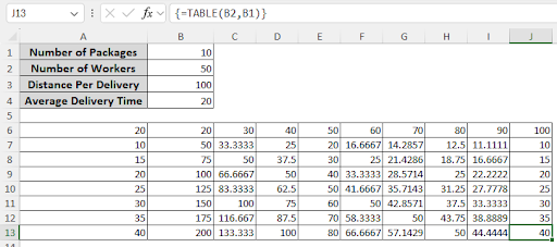
Finally, Excel will populate the entire data table, showing you the Profit for every combination of number of packages and number of workers. This provides a comprehensive overview of how these two variables collectively influence the average delivery time.
Three Variable Sensitivity Analysis
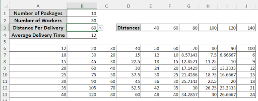
While a two-variable Data Table is excellent for analyzing two changing inputs, sometimes you need to consider a third variable. You can achieve this by combining a two-variable data table with a data validation list, allowing you to dynamically change a third input and observe its impact on the table’s results. Here, we will make the distance per delivery our third variable.
➤ First, we need to create a list of different average distances per delivery that we can use as a variable.
Here, we start from E3 with 40 miles, then end with 140 in the J3 cell.
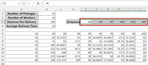
➤ We are using the two-variable data table from the previous method so that it becomes easier for you to follow.
➤ Click on the B3 cell, and from the Data tab, go to Data Tools > Data Validation.
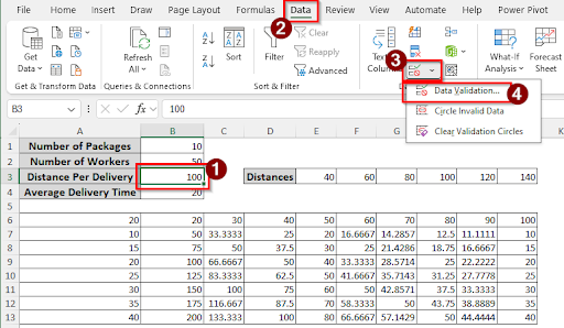
➤ Select the cell where you want your dropdown list to appear (cell F2).
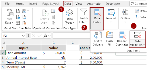
➤ Navigate to the Data tab in the Excel ribbon.
➤ In the Data Tools group, click on Data Validation.
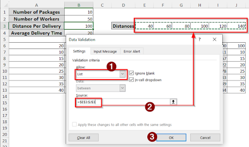
➤ In the Data Validation dialog box, under the “Settings” tab:
From the “Allow” drop-down, select List.
In the “Source” field, input the range containing your list of distances, which is =$E$3:$J$3.
➤ Click OK.
Thus, a drop-down arrow will appear in cell B3, allowing you to select different distances from your predefined list.
➤ Choose a distance from the drop-down list.
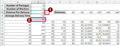
Finally, as you select different distances from the drop-down list in cell B3, your entire two-variable data table will dynamically update. This will show you the average delivery time in minutes based on the chosen number of packages, workers, and distance in miles per delivery.
Downloadable Resources
Get our practice workbook or necessary files that we have worked with to prepare this article.
What-if Analysis in Excel.xlsx
Frequently Asked Questions
How to fix if Goal Seek is not working in Excel?
You can increase the Maximum Iterations or reduce the Maximum Change from File > Options > Formulas to improve accuracy and find better solutions.
What is the difference between Scenario Manager and Data Table?
Scenario Manager lets you save and switch between multiple input sets manually, while Data Tables automatically calculate and display results based on varying inputs.
Is there a limit to how many scenarios I can create?
Excel allows up to 32 changing cells per scenario and up to 255 scenarios in a worksheet.
Concluding Words
Above, we have explored all the essential methods to perform what-if analysis in Excel, including Scenario Manager, Goal Seek, and Data Tables. These tools help you test different inputs, analyze outcomes, and make better-informed decisions. With these techniques, you can model, plan, and forecast more effectively right within Excel. If you have any questions, feel free to share them in the comment section below.