

When working with financial models or business data in Excel, it’s important to understand how small changes in key variables can impact your results. That is where sensitivity analysis comes in. It allows you to test different values and see how they impact your outcome, without changing your original model. In this guide, we will walk you through how to perform sensitivity analysis in Excel using tools like Data Tables, Goal Seek, and Solver.
To use sensitivity analysis with Goal Seek in Excel, follow the steps below.
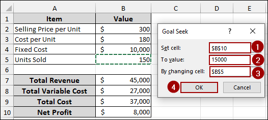
➤ Go to the Data tab, click What-If Analysis, and choose Goal Seek.
➤ In the Goal Seek dialog box:
For “Set cell“, select the cell that contains your target outcome, which is B10 (Net Profit).
For “To value“, enter your desired net profit, which is $15000.
For “By changing cell“, select the input cell that Goal Seek should adjust to reach your target.
➤ Press OK, and Excel will automatically change the input(cell B5) to 150 to reach your goal with net profit of $15,000(cell B10).
What is Sensitivity Analysis?
Sensitivity analysis is a method used to evaluate how different values of input variables affect the output. In Excel, it helps you test various what-if scenarios by changing one or more inputs and observing how those changes impact your results. This technique is especially useful in business, finance, and forecasting, where decision-making often depends on uncertain or variable factors.
Using Data Table for Sensitivity Analysis
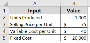
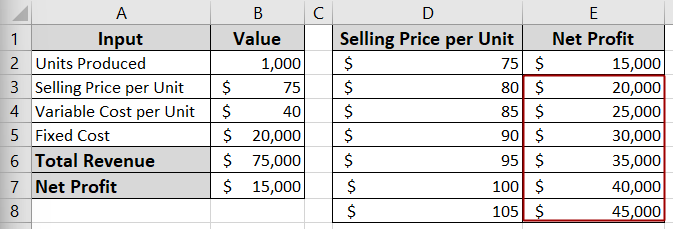
In this section, we will perform a sensitivity analysis using the Data Table for a business profit model. Suppose we have a dataset with the following inputs: Units Produced: 1,000 (in cell B2), Selling Price per Unit: $75 (in cell B3), Variable Cost per Unit: $40 (in cell B4), and Fixed Cost: $20,000 (in cell B5). Here, we will examine how changing one variable (Selling Price per Unit) and two variables (Selling Price per Unit and Units Produced) affect the Net Profit.
One Variable Sensitivity Analysis
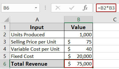
First, we will calculate the Total Revenue. To do so,
➤ Select cell B6, put the following formula, and press ENTER.
=B2*B3
This will calculate the Total Revenue by multiplying the Units Produced by the Selling Price per Unit.
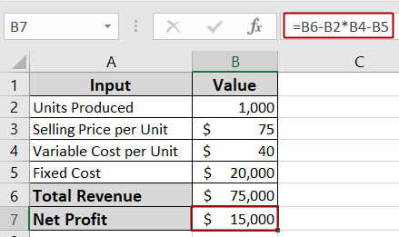
Next, we will calculate the Net Profit.
➤ Select cell B7, enter the following formula, and press ENTER.
=B6-B2*B4-B5
This will calculate the Net Profit by subtracting the Total Variable Cost and Fixed Cost from the Total Revenue.
Now, let’s create the structure for our sensitivity analysis data table.
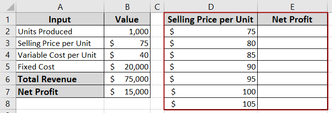
➤ In cell D1, enter “Selling Price per Unit” and in cell E1, enter “Net Profit”.
➤ Below “Selling Price per Unit”, list the different selling prices you want to analyze, for example, from $75 to $105 in column D.
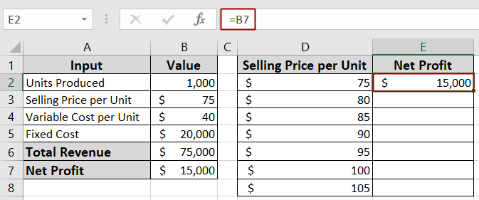
➤ Enter the formula in cell E2 and press ENTER.
=B7
This ensures the data table references your original Net Profit calculation.
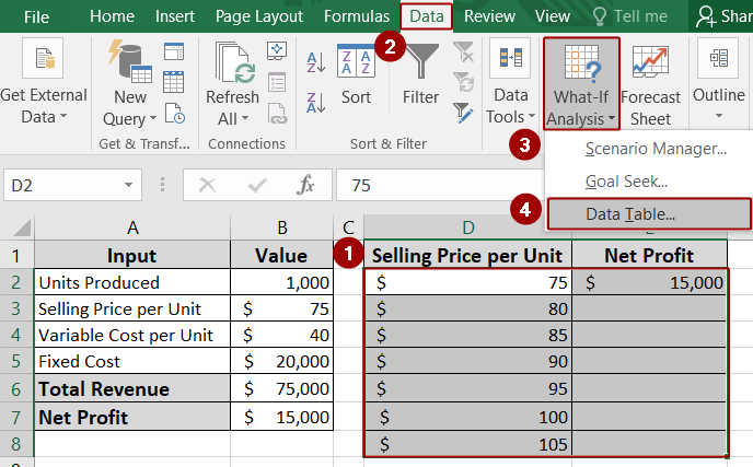
➤ Select cells D2 to E8, containing the different Selling Price per Unit values and the Net Profit formula reference.
➤ Navigate to the Data tab in the Excel ribbon.
➤ Click on What-If Analysis.
➤ From the drop-down menu, select Data Table.
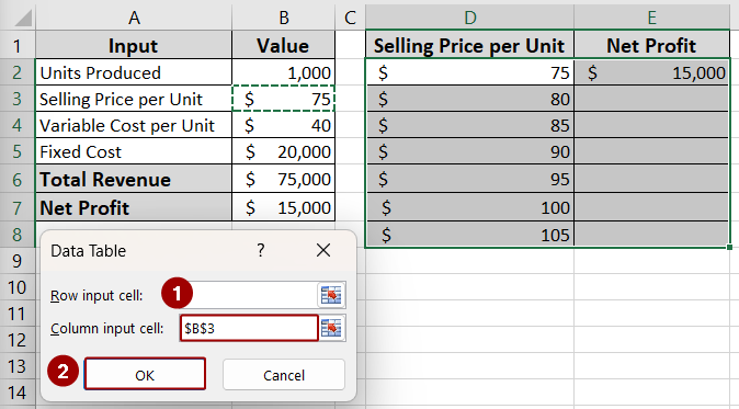
This will open the Data Table dialog box.
➤ In the Data Table dialog box:
Leave “Row input cell” blank, as our varying input values are arranged in a column.
For “Column input cell“, select the cell that holds your original Selling Price per Unit, which is B3.
This tells Excel to substitute the values from column D into cell B3 to calculate the corresponding Net Profit.
➤ Click OK.
Finally, the data table will populate, showing the calculated Net Profit for each Selling Price per Unit. For example, when the Selling Price per Unit is $75, the Net Profit is $15,000. As the selling price increases, the Net Profit also increases, reaching $45,000 at a Selling Price per Unit of $105.
Two Variable Sensitivity Analysis
Two variable sensitivity analysis lets you examine how changes in two input variables affect a single output in your model. In this part, we will demonstrate how changing “Selling Price per Unit” and “Units Produced” simultaneously impacts the “Net Profit”.
Just like the previous data, ensure your “Units Produced”, “Selling Price per Unit”, “Variable Cost per Unit”, and “Fixed Cost” inputs are set up. The “Total Revenue” in cell B6 and “Net Profit” in cell B7 should also be calculated using the formulas shown earlier.
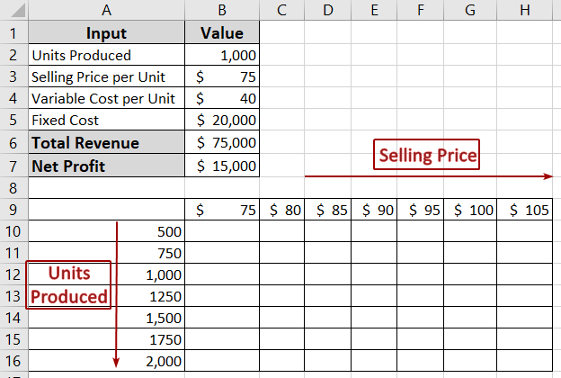
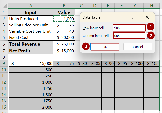
Now, let’s prepare the grid for our two-variable data table. Along the top row, starting from cell B9 and moving rightward, list the different Selling Price per Unit values you want to analyze, such as $75, $80, $85, $90, $95, $100, and $105.
Down the first column, starting from cell A10 and moving downward, list the different Units Produced values you want to analyze, such as 500, 750, 1,000, 1,250, 1,500, 1,750, and 2,000.
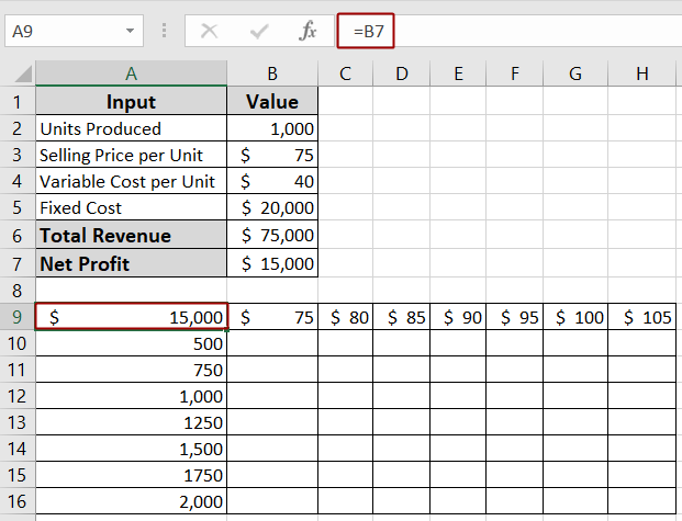
➤ In cell A9, link this cell to your “Net Profit” by entering the formula.
=B7
This is the intersection point for your two varying inputs.
➤ Select cell A9 and go to the Data tab in the Excel ribbon.
➤ In the Forecast group, click on What-If Analysis.
➤ From the drop-down menu, select Data Table.
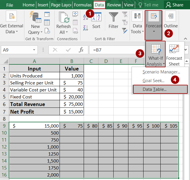
This will open the Data Table dialog box.
➤ In the Data Table dialog box:
For “Row input cell“, select the cell that holds your original Selling Price per Unit, which is B3.
This tells Excel to substitute the values from the top row into cell B3.
For “Column input cell“, select the cell that holds your original Units Produced, which is B2.
This tells Excel to substitute the values from the first column into cell B2.
➤ Click OK.
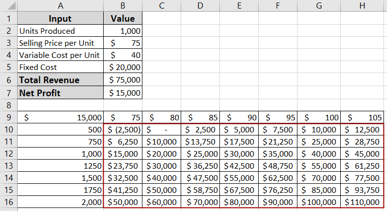
Finally, Excel will generate the entire two-variable data table, showing the “Net Profit” for every combination of “Selling Price per Unit” and “Units Produced”. For example, producing 500 units at a Selling Price per Unit of $75 results in a Net Profit of -$2,500, while producing 2,000 units at a Selling Price per Unit of $105 results in a Net Profit of $110,000.
Applying Goal Seek for Sensitivity Analysis
Goal Seek is a built-in Excel tool that helps you find the right input value to get a specific result. It’s useful in sensitivity analysis when you want to see how changing one input affects your outcome.
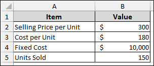
Suppose we have a dataset containing various components like Selling Price per Unit as $300, Cost per Unit as $180, Fixed Cost as $10,000, and Units Sold as 150. Here, we will calculate how many units we need to sell to reach a net profit of $15000.
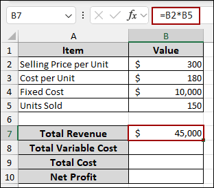
➤ In cell B7, enter the formula.
=B2*B5
It will calculate the Total Revenue by multiplying the Selling Price per Unit by the Units Sold.
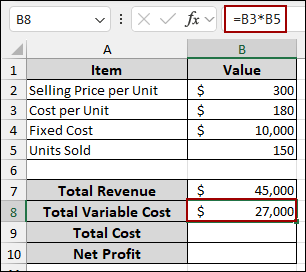
➤ In cell B8, enter the formula below.
=B3*B5
This will determine the Total Variable Cost by multiplying the Cost per Unit by the Units Sold.
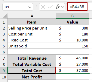
➤ In cell B9, write down the following formula.
=B4+B8
This way, we will get the Total Cost by summing the Fixed Cost and the Total Variable Cost.
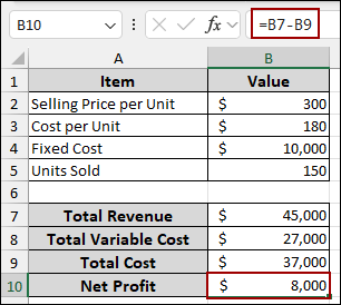
➤ In cell B10, insert the formula.
=B7-B9
Thus, computing the Net Profit by subtracting the Total Cost from the Total Revenue.
Now, we will perform a sensitivity analysis using the Goal Seek feature. This will help us determine the Units Sold needed to achieve a target Net Profit of $15,000.
➤ Navigate to the Data tab from the menu bar.
➤ Click on What-If Analysis in the Forecast group.
➤ Select Goal Seek from the drop-down menu.
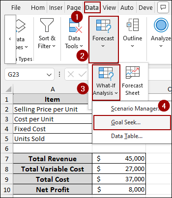
The Goal Seek dialog box will appear.
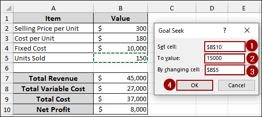
➤ In the Set cell field, enter B10. This is our Net Profit cell.
➤ In the To value field, type 15000. This is our target profit.
➤ In the By changing cell field, enter B5. This is the cell representing Units Sold that we want to change.
➤ Finally, click OK.
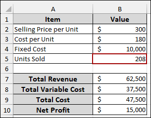
As a result, Excel will calculate the necessary Units Sold (approximately 208) to reach a Net Profit of $15,000, and the values in your spreadsheet will update accordingly.
Using Solver for Sensitivity Analysis
Solver is an advanced Excel tool that lets you find the best possible result by changing multiple inputs while following specific rules or limits. In sensitivity analysis, you can use Solver to maximize profit, minimize cost, or meet a target value by adjusting several variables at once. Here, we will use Solver to find the best combination of Mountain and Road bikes that maximizes total profit, while staying within the limits of available labor hours and materials.
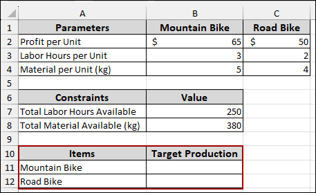
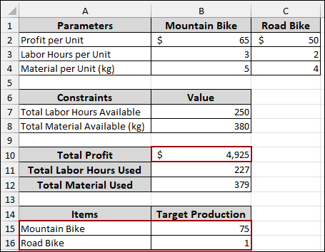
Suppose we have a dataset of Parameters, Constraints, and Target Production for Mountain Bikes and Road Bikes.
Here are the Parameters for both Mountain Bike and Road Bike:
Profit per Unit: $65 (Mountain Bike), $50 (Road Bike)
Labor Hours per Unit: 3 (Mountain Bike), 2 (Road Bike)
Material per Unit (kg): 5 (Mountain Bike), 4 (Road Bike)
For the Constraints:
Total Labor Hours Available: 250
Total Material Available (kg): 380
Below, we have an “Items” section with “Mountain Bike” and “Road Bike” to define the Target Production.
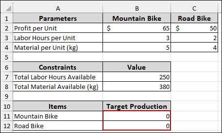
➤ First, set the values to 0 for “Mountain Bike” and “Road Bike” in the “Items” section.
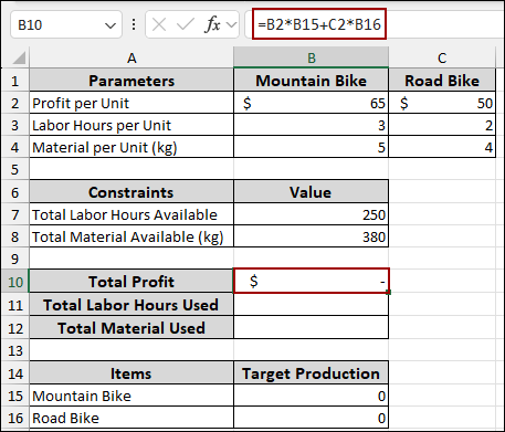
Now, we will calculate the Total Profit based on the number of units produced for each bike type.
➤ In cell B10, put the formula down.
=B2*B15+C2*B16
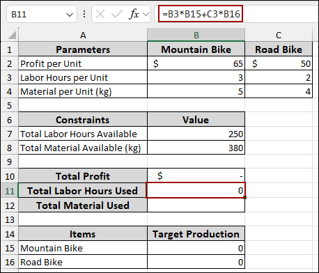
Next, we will determine the Total Labor Hours Used for production.
➤ In cell B11, input the formula.
=B3*B15+C3*B16
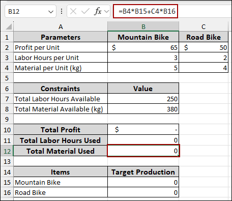
Similarly, we will calculate the Total Material Used during the production process.
➤ In cell B12, enter the formula.
=B4*B15+C4*B16
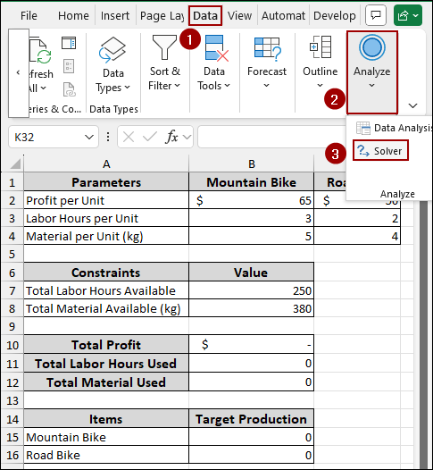
Now, we will use the Solver add-in to determine the optimal production of Mountain Bikes and Road Bikes to maximize Total Profit while adhering to labor and material constraints.
➤ Go to the Data tab in the Excel ribbon.
➤ In the Analyze group, click on Solver.
The Solver Parameters dialog box will appear.
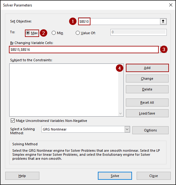
➤ In the Set Objective field, select cell B10 (Total Profit).
➤ Choose Max to maximize the profit.
➤ In the By Changing Variable Cells field, select cells B15 and B16 (Target Production for Mountain Bike and Road Bike).
Now, we need to add the constraints.
➤ Click the Add button next to “Subject to the Constraints“.
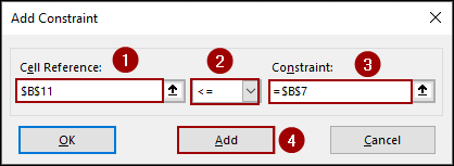
A new Add Constraint dialog box will open. Here, we will add a labor hour constraint.
➤ In the Cell Reference box, select cell B11 (Total Labor Hours Used).
➤ From the dropdown, choose the <= operator.
➤ In the Constraint box, select cell B7 (Total Labor Hours Available).
➤ Click Add to add this constraint.
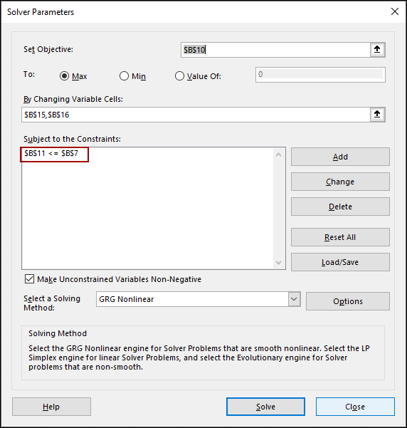
As you can see, we have successfully added the constraints in the Solver Parameters.
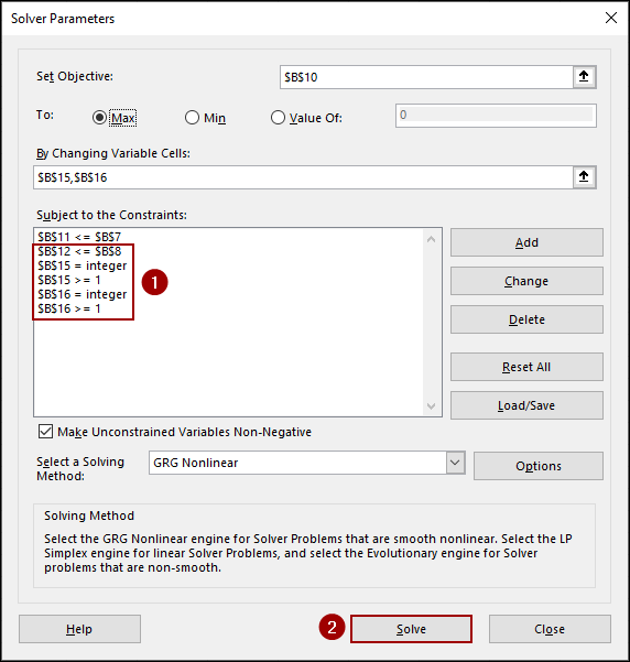
➤ Similarly, we will add the rest of the constraints in the box.
For Cell Reference B11, choose the <= operator. In the Constraint box, select cell B7.
For Cell Reference: B15, choose int (integer).
For Cell Reference: B16, choose int (integer).
For Cell Reference: B15, choose >= and enter 1 in the Constraint box.
For Cell Reference: B16, choose >= and enter 1 in the Constraint box.
➤ After adding all the constraints, finally, click Solve.
As a result, the Target Production values in cells B15 and B16 will update to show the optimal number of Mountain Bikes and Road Bikes to produce, which will also maximize the Total Profit in cell B10 while respecting all your defined constraints.
Downloadable Resources
Get our practice workbook or necessary files that we have worked with to prepare this article.
Sensitivity Analysis in Excel.xlsx
Frequently Asked Questions
What is the difference between what-if analysis and sensitivity analysis in Excel?
What-if analysis is a broader term that includes tools like Scenario Manager, Goal Seek, and Data Tables. Sensitivity analysis is a specific type of what-if analysis that focuses on how changes in input variables affect your model’s outcome.
Can I use Goal Seek for multiple variables?
No, Goal Seek can only change one input cell to reach a desired result. If you need to adjust multiple variables, use the Solver tool instead.
Do I need to enable Solver manually in Excel?
Yes, Solver is not enabled by default. Go to File > Options > Add-ins > Excel Add-ins > Go, then check the box for Solver Add-in and click OK.
Concluding Words
Above, we have covered the key techniques to perform sensitivity analysis in Excel, including one-Variable and two-Variable Data Tables, Goal Seek, and Solver. These methods help you understand how changes in your inputs affect the results. Whether you’re analyzing profits, costs, or any other outcome, sensitivity analysis gives you a clear picture of your model’s behavior. If you have any questions, feel free to share them in the comment section below.