How to Show Columns Side by Side in Excel Pivot Table

Pivot Tables are a powerful tool for summarizing data in Excel. However, when you drag multiple fields into the Rows area, Excel’s default layout (Compact Form) nests them together. This makes your data hard to read. Fortunately, you can change this layout to display your columns side by side. In this article, we will walk you through several methods to show columns side by side.

This is the most straightforward method due to its clean and readable format. It displays each row field in its own column, giving you a classic, spreadsheet-like view.

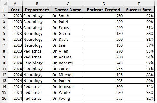
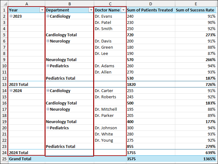
Imagine we have some sample data that includes Year, Department, Doctor Name, Patients Treated, and Success Rate. Now, we will create a Pivot Table to view how the fields are initially nested and then apply the Tabular Form to display columns side by side.

To create the Pivot Table:

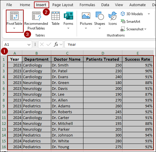
➤ Select your dataset, and go to Insert > PivotTable.
➤ In the new window, choose New Worksheet and click OK.

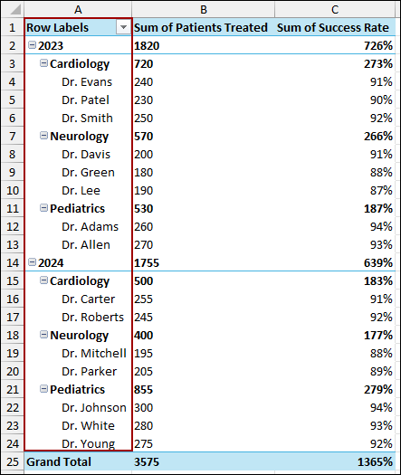
As a result, your new Pivot Table will appear. By default, with multiple fields in the Rows area, you will see Department and Doctor Name nested under Year.

Now, let’s change the layout:

➤ Click anywhere inside your Pivot Table.
➤ Go to the Design tab on the ribbon.
➤ In the Layout group, click Report Layout.
➤ From the dropdown menu, select Show in Tabular Form.

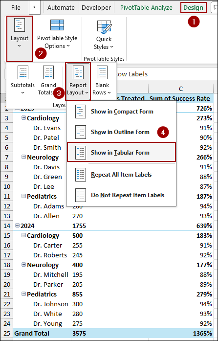
Your Pivot Table will instantly change to a tabular format, showing each field in its own column.

Similar to the Tabular Form, the Outline Form also separates your nested fields into individual columns. Here, we will use the Outline Form to show columns side by side. The main difference lies in where it places the subtotals.

➤ Select your Pivot Table.
➤ Navigate to the Design tab.
➤ In the Layout group, click Report Layout.
➤ Choose Show in Outline Form from the dropdown menu.

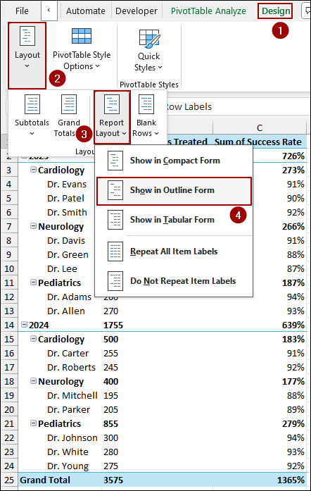
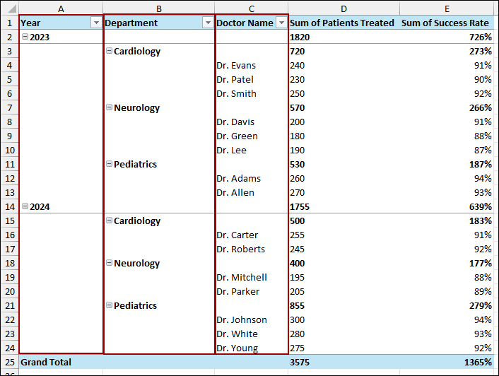
As a result, your Pivot Table will change to Outline Form layout to show columns side by side. You will also notice how the subtotals are now at the top of each group instead of the bottom.

If you are using the older Excel versions, the Classic PivotTable layout is a great option to display columns side by side. It offers a slightly different interface and allows you to drag fields directly within the Pivot Table grid to rearrange them.

To enable the Classic Pivot Table layout:

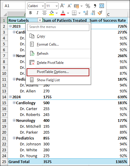
➤ Right-click anywhere on your Pivot Table.
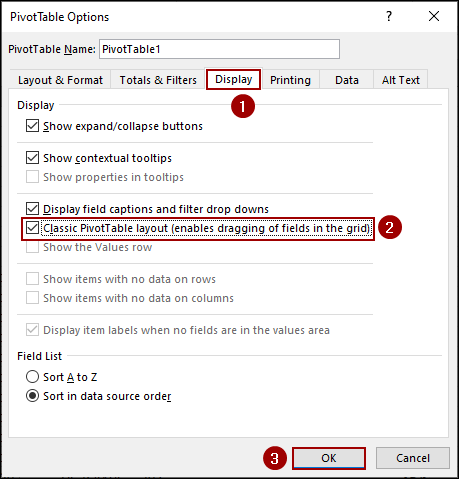
➤ From the context menu, select PivotTable Options.

➤ In the PivotTable Options dialog box, go to the Display tab.
➤ Check the box for Classic PivotTable layout (enables dragging of fields in the grid).
➤ Click OK.

Thus, your Pivot Table will now be in the classic format, with each row field in its own column. This layout also provides a lot of flexibility for reorganizing your data.

For a more automated approach, you can use a simple VBA macro to change the Pivot Table layout. This is useful if you regularly create Pivot Tables and want to set the layout with a single click.

➤ Go to the Developer tab, and click Visual Basic.

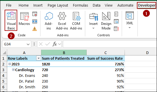
➤ In the VBA editor, click Insert > Module and paste the following code.

Sub PivotColumnsSideBySide()
Dim ws As Worksheet
Dim pivot As PivotTable
Set ws = ThisWorkbook.Sheets("VBA")
Set pivot = ws.PivotTables("PivotTable1")
pivot.RowAxisLayout xlTabularRow
End Sub

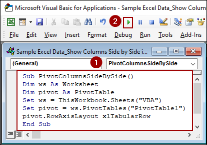
This will automatically change your Pivot Table’s layout to the Tabular Form, achieving the side-by-side column view.

Frequently Asked Questions

Can I keep column headers visible when showing columns side by side?

Yes, enable Repeat All Item Labels from Pivot Table Options > Design > Report Layout to keep headers visible for each row.

Why does my Pivot Table merge columns instead of showing them separately?

This usually happens if the same field is placed in both Rows and Columns areas or if the layout is in Compact Form. Remove duplicates or change the layout.

Why do my columns collapse after refreshing the Pivot Table?

Pivot Tables often reset to the default layout (Compact Form) after refresh. To prevent this, set the layout to Tabular Form and checkmark “Preserve cell formatting on update” in Pivot Table Options.

Concluding Words

Above, we have explored all the methods to display columns side by side. By changing the Report Layout to Tabular or Outline Form, you can quickly change the layout of your Pivot Table. The Classic layout is a great alternative that provides more flexibility, while a simple VBA macro can automate the process. If you have any other questions about Pivot Tables or Excel, feel free to ask them in the comments section below.