How to Show Text in Values Area of Excel Pivot Table

In an Excel PivotTable, by default, the Values area only displays numerical data. Sometimes you might need to show text instead of values. By adding new measures or using format cells, you can display text in the Values section. In this article, we will walk you through two effective methods to display text in the Values section of a Pivot Table.

This method is useful as it allows you to concatenate multiple text values into a single cell. Here, we will add a new measure, use the CONCATENAX function, and then add the measure in the Values section to show text instead of numeric values.

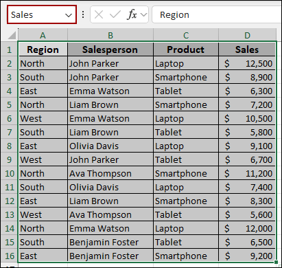
Imagine we have a sample dataset containing Region, Salesperson, Product, and Sales.

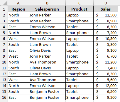
Before starting, we have named the data range as Sales.

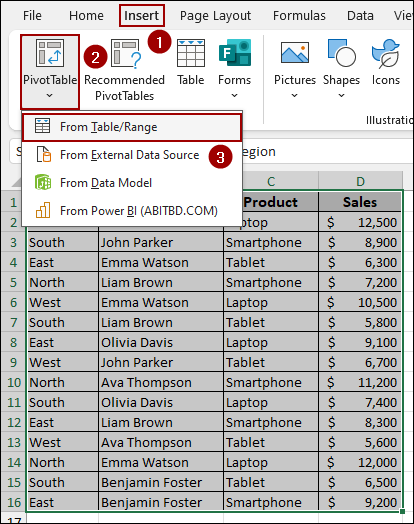
Now, let’s create the Pivot Table. For that,

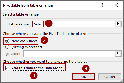
➤ Go to Insert > PivotTable > From Table/Range.

➤ In the PivotTable from table or range window, select New Worksheet.
➤ Make sure you checkmark the box for “Add this data to the Data Model“.
➤ Click OK.

Now, your Pivot Table will be created.

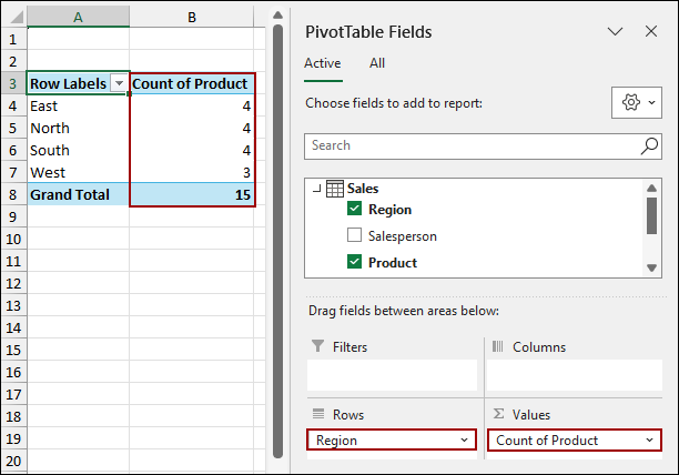
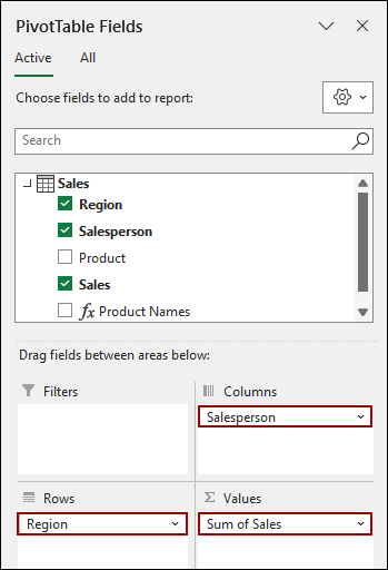
➤ Drag Region to the Rows area.
➤ Then, drag Product to the Values area.

Excel will automatically apply a COUNT function to the text field, showing you the number of products sold in each region.

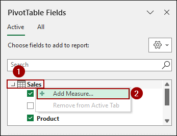
To show the actual product names, we need to create a Measure. For this,

➤ In the PivotTable Fields pane, right-click on your table name (in this case, it is “Sales”).
➤ From the context menu, select Add Measure.

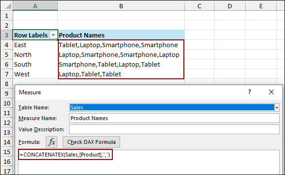
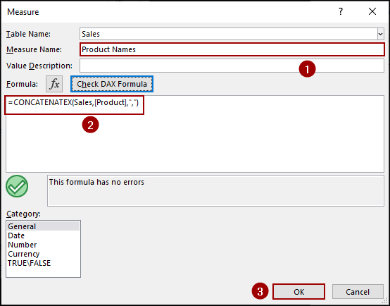
In the Measure window.

➤ Give your measure a name, like “Product Names.”
➤ In the Formula box, paste the following DAX code.

➤ Click OK.

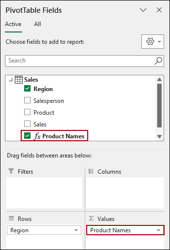
Now, in the PivotTable Fields list, you will see your new measure, Product Names.

➤ Drag the Product Names measure to the Values area.

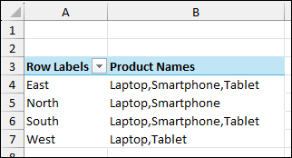
Your Pivot Table will now display the names of all products sold in each region, separated by a comma.

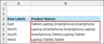
Here, you might notice that there are duplicates in the list. To fix this, you need to modify the DAX formula to show unique values.

➤ Right-click the Product Names measure and select Edit Measure.

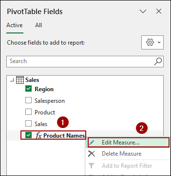
➤ Change the formula and click OK.

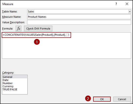
As a result, your Pivot Table will now show a list of unique products sold per region.

This method is ideal when you want to replace numerical values with text based on specific conditions. Here, we will use the Format Cells feature to show numerical values as text. To start with, we will use the same Pivot Table summarizing sales data.

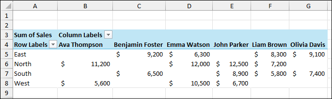
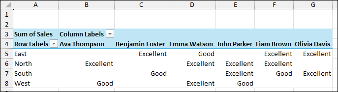
➤ Drag Region to the Rows area, Salesperson to the Columns area, and Sales to the Values area.

Thus, your Pivot Table will be rearranged just like the one below.

To replace the sales numbers with text, we will use a custom number format.

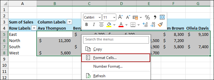
➤ Select cells in the values section of your Pivot Table.
➤ From the context menu, select Format Cells.

The Format Cells dialog box will appear.

➤ Go to the Number tab.
➤ Select Custom from the category list.
➤ In the Type box, enter the following code.
[>7000]”Excellent”;”Good”
➤ Click OK.

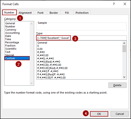
This code tells Excel to display “Excellent” if the value is greater than 7000 and “Good” if it is not. Your Pivot Table will now show text instead of numbers in the Values section.

Frequently Asked Questions

Why does my Pivot Table show “blank” instead of the text I want?

This happens when the field used in the Values area contains text and no numeric aggregation can be applied. Replace blanks with meaningful placeholders or use a helper column.

Can I use a custom calculation to display text in Pivot Tables?

No, custom calculations (like calculated fields) still require numeric data. To show text, you need to prepare your data first using formulas or Format Cells.

Can I sort or filter a Pivot Table based on the displayed text?

Yes, once text is displayed, you can sort alphabetically or filter by text normally.

Concluding Words

Above, we have explored all the methods to display text in the Values section of a Pivot Table. By using the CONCATENAX function, you can easily list text values instead of numerical values. Alternatively, the Format Cells feature is a simple yet effective way to categorize your numerical data with custom texts. If you have any other questions about Pivot Tables or Excel, feel free to ask them in the comments section below.