A Pivot Table is a useful tool in Excel for organizing large datasets. By default, when you add multiple fields to the Rows area, Excel displays them in a Compact Form, which nests them in a single column. This layout can make your data difficult to read, especially with many fields. Fortunately, Excel offers a Tabular Form layout that represents each field in its own separate column. In this article, we will guide you through several methods to display your Pivot Table in a tabular format.
To show a Pivot Table in Tabular Form, here is one simple solution by changing the layout.
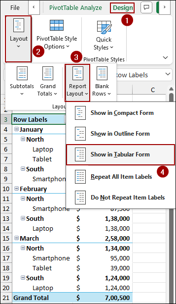
➤ Click anywhere inside your Pivot Table and go to the Design tab on the ribbon.
➤ In the Layout group, click Report Layout.
➤ From the dropdown menu, select Show in Tabular Form to display the Pivot Table in Tabular Form.

Using Report Layout Feature to Enable Tabular Form
This is the most common method to change your Pivot Table’s layout. It works better when you need a quick, readable view of your data with each field in its own column.
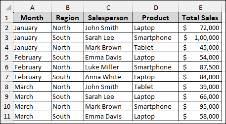
Imagine a sample sales-related dataset containing information on Month, Region, Salesperson, Product, and Total Sales. Now, we will create a Pivot Table and then use the Show in Tabular Form feature from the Report Layout list.
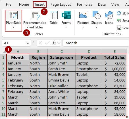
➤ Select your dataset.
➤ Go to Insert > PivotTable.
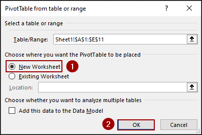
➤ In the new window, choose New Worksheet and click OK.
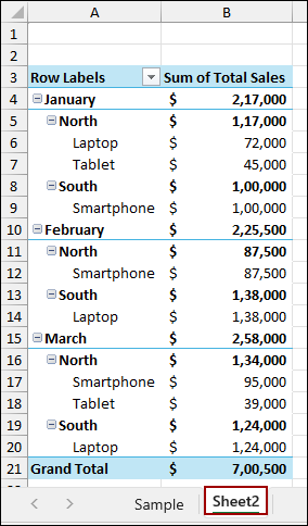
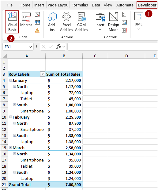
The new Pivot Table will appear in a new sheet named Sheet2. By default, with multiple fields in the Rows area, you will see them nested in a single column. For our example, if we place Month, Region, and Product in the Rows area, they will appear nested together.
Now, let’s change the layout to Tabular Form.
➤ Click anywhere inside your Pivot Table.
➤ Go to the Design tab on the ribbon.
➤ In the Layout group, click Report Layout.
➤ From the dropdown menu, select Show in Tabular Form.
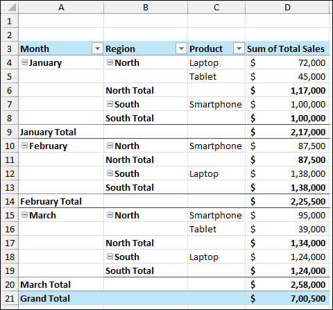
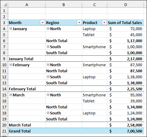
Thus, your Pivot Table will instantly change to a tabular layout, showing each field in its own column.
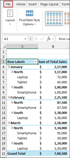
If you want Tabular Form as the default layout for your Pivot Table, you can change the layout from the Data option.
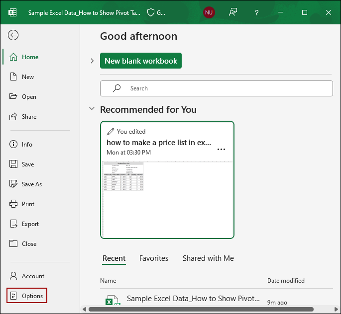
➤ Click the File option from the ribbon.
➤ Hit the Options button from the bottom.
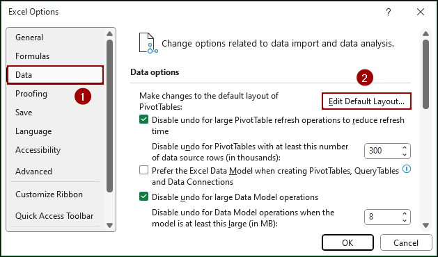
➤ Now, choose Data and click Edit Default Layout.
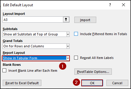
➤ From the Report Layout drop-down menu, select Show in Tabular Form and click OK.
This change will ensure that every new Pivot Table you create will automatically have its fields displayed in separate columns.
Using Field Settings Option
Another way to achieve the tabular layout is by using the Field Settings for each field individually. This method gives you more advanced control over the layout of each field within your Pivot Table.
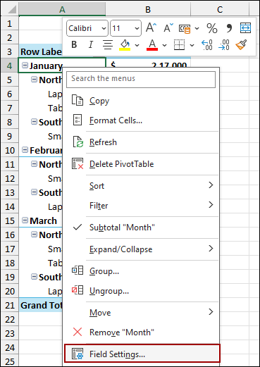
➤ Right-click any cell in the Pivot Table that contains a row label.
➤ From the context menu, select Field Settings.
➤ In the Field Settings dialog box, go to the Layout & Print tab.
➤ Under the Layout section, select the radio button for Show item labels in tabular form.
➤ Click OK.
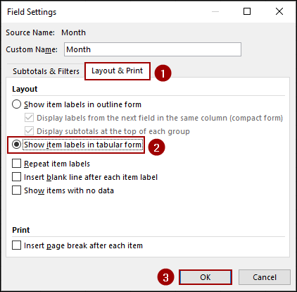
As a result, the selected field (in this case, Month) will now appear in its own column, and the Pivot Table will adopt the tabular layout. Repeat the process for other row labels to show all the columns in Tabular Form.

Embedding VBA Code to Display as Tabular Format
For a more automated approach, you can use a simple VBA macro to change the Pivot Table layout. This is useful if you want a one-click solution to set the layout to tabular form.
➤ Go to the Developer tab, and click Visual Basic.
➤ In the VBA editor, click Insert > Module.
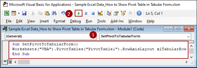
➤ In the new module, paste the following code and hit Run.
Sub SetPivotToTabularForm()
Worksheets("VBA").PivotTables("PivotTable1").RowAxisLayout xlTabularRow
End Sub
Note:
You might need to change “VBA” to the name of your worksheet and “PivotTable1” to the name of your Pivot Table.
This will automatically change your Pivot Table’s layout to the Tabular Form, achieving the side-by-side column view with a single click.
Frequently Asked Questions
Does Tabular Form affect the Pivot Table calculations?
No, it only changes the layout. All summaries, totals, and calculations remain the same.
How do I remove blank rows that appear after switching to Tabular Form?
You can either filter out blank values or remove them using PivotTable Options > Layout & Format > For empty cells show.
Why does my Tabular Form Pivot Table look messy when exporting to Excel or PDF?
Sometimes merged cells or hidden subtotals create formatting issues. To fix this, remove subtotals and repeat item labels for a clean export.
Concluding Words
Above, we have explored several methods to display your Pivot Table in tabular format. Whether you choose the straightforward Show in Tabular Form feature, use the more specific Field Settings, or automate the process with a simple VBA macro, each method helps transform your data into a clean tabular view. If you have any other questions about Pivot Tables or Excel, feel free to ask them in the comments section below.