Sometimes you might need to analyze different business outcomes under varying conditions. The Scenario Manager in Excel helps you test multiple what-if scenarios. You can also combine this with a Pivot Table, which allows you to create a summarized report. In this article, we will walk you through the process of creating a Scenario Pivot Table report in Excel using three simple steps.
To create a scenario Pivot Table report in Excel, here is one simple solution by using the Scenario Pivot Table report feature.
➤ Create a dataset that includes all the key variables and a formula that calculates the final outcome, like profit.
➤ Use the Scenario Manager feature to define different scenarios (e.g., Best Case, Worst Case) by inputting new values for your changing cells.
➤ Click on Summary > Scenario Pivot Table Report to create a scenario Pivot Table report.
Steps to Create a Scenario Pivot Table Report in Excel
Here, we will go through several steps to create a scenario Pivot Table report in Excel.
Step 1: Creating Dataset
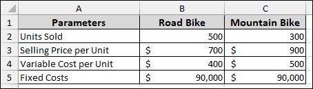
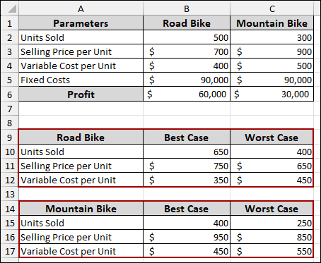
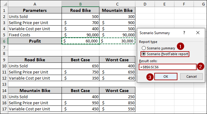
In this first step, we will create a dataset for our analysis. Imagine we have a sample dataset containing Parameters in column A. In cells A2 to A5, we have the variables “Units Sold”, “Selling Price per Unit”, “Variable Cost per Unit”, and “Fixed Costs”.
In cells B2 to B5, we have the data for the “Road Bike” (e.g., 500 units, $700 selling price, $400 variable cost, and $90,000 fixed costs).
Similarly, in cells C2 to C5, for the “Mountain Bike” (e.g., 300 units, $900 selling price, $500 variable cost, and $90,000 fixed costs).
Now, let’s calculate the Profit for each product.
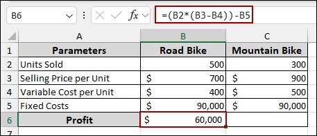
➤ In cell B6, write down the formula to calculate the profit for the Road Bike.
=(B2*(B3-B4))-B5
This formula multiplies the units sold by the profit per unit (selling price minus variable cost) and then subtracts the fixed costs.
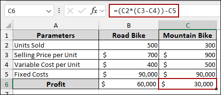
➤ Next, in cell C6, enter the formula for the Mountain Bike.
=(C2*(C3-C4))-C5
The profit for the Mountain Bike will now be displayed in cell C6.
For the scenario analysis, we need different case values. Below the main dataset, outlining the “Best Case” and “Worst Case” values for “Units Sold,” “Selling Price per Unit,” and “Variable Cost per Unit” for both the Road and Mountain Bikes. This table will be our reference when defining the scenarios.
Step 2: Applying Scenario Manager Feature
In the next step, we will use the Scenario Manager to create different scenarios based on the “Best Case” and “Worst Case” values.
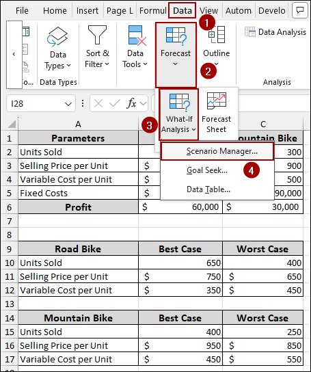
➤ Navigate to the Data tab on the ribbon.
➤ In the Forecast group, click on What-If Analysis.
➤ From the dropdown menu, select Scenario Manager.
➤ In the Scenario Manager dialog box, click the Add button to create your first scenario.
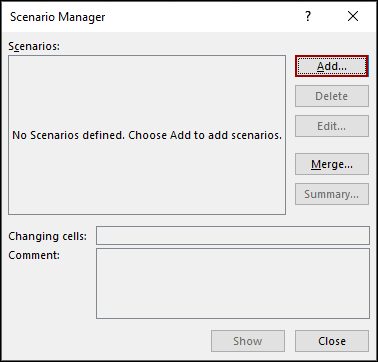
A new dialog box named Edit Scenario will appear.
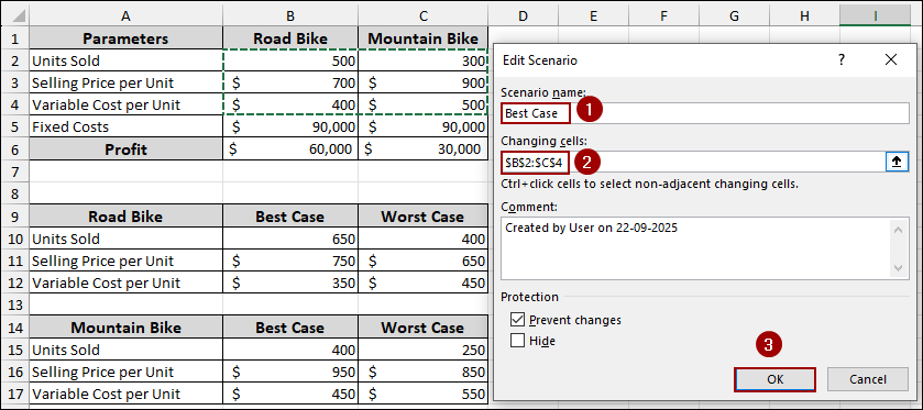
➤ In the Scenario name field, type “Best Case”.
➤ In the Changing cells field, select the range containing the values for units sold, selling price, and variable cost for both bikes, which is B2:C4.
➤ Click OK.
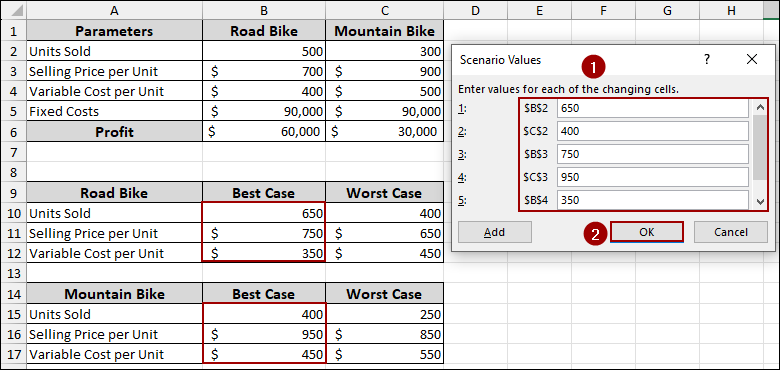
The Scenario Values dialog box will pop up.
➤ Enter the values for your “Best Case” scenario, referencing the table you created in Step 1. For example, for Road Bike, enter 650 for units sold, 750 for selling price, and 350 for variable cost. For Mountain Bike, enter 400 for units sold, 950 for selling price, and 450 for variable cost.
➤ Click OK.
Thus, the best-case scenario will be added. Now, we will create the worst-case scenario.
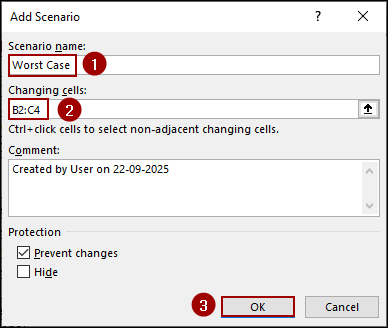
➤ In the Scenario Manager dialog box, click Add again.
➤ In the Add Scenario dialog box, name the new scenario “Worst Case”.
The Changing cells should remain B2:C4.
➤ Click OK.
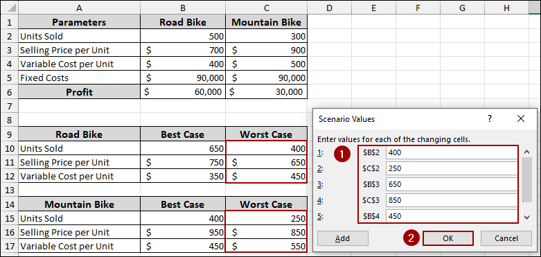
➤ Enter the “Worst Case” values for both products, again referencing your reference table.
➤ Click OK.
Step 3: Making Scenario Pivot Table Report
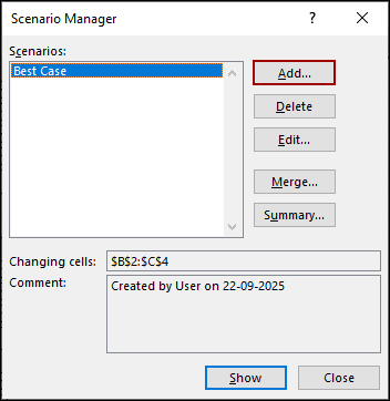
In this final step, we will create an easy-to-read report using a Pivot Table to summarize the results of our scenarios. Here, we have both “Best Case” and “Worst Case” scenarios listed in the Scenario Manager dialog box.
➤ In the Scenario Manager dialog box, click the Summary button.
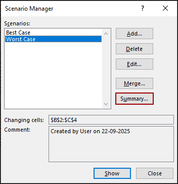
The Scenario Summary dialog box will appear.
➤ Under Report type, select Scenario PivotTable report.
➤ In the Result cells field, select the range containing your profit calculations, which is B6:C6.
➤ Click OK.
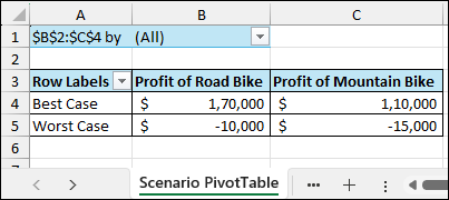
Excel will automatically generate a new worksheet containing a Scenario Pivot Table Report. This report shows a side-by-side comparison of the profit for each product under both “Best Case” and “Worst Case” scenarios. Finally, we have successfully created a scenario Pivot Table report in Excel.

Frequently Asked Questions
What is the difference between a Scenario Summary and a Scenario Pivot Table Report?
A Scenario Summary creates a static table of results, while a Scenario Pivot Table Report creates an interactive report that you can filter and pivot like a regular Pivot Table.
How can I modify a scenario?
You can modify an existing scenario by selecting its name in the Scenario Manager dialog box and clicking the Edit button.
Can I update the Scenario Pivot Table Report automatically if my scenario values change?
No, the Scenario Pivot Table Report is static. If you change scenario inputs, you will need to regenerate the report by going back to Scenario Manager > Summary.
Concluding Words
Above, we have covered all the steps to create a scenario Pivot Table report in Excel. Unlike a regular summary, the PivotTable report allows more features like filters, slicers, and field arrangements. Whether you are evaluating best-case, worst-case, or custom scenarios, this report helps you create a more dynamic report. If you have any questions, feel free to share them in the comment section below.