Create Pivot Table from Multiple Sheets with Same Columns

If you have data spread across multiple worksheets with the same columns, creating a single PivotTable can be a challenge. Manually combining the data by copying and pasting can be a time-consuming task. Fortunately, Excel offers several built-in tools to create a single Pivot Table from multiple sheets.

In this article, we will walk you through three effective methods to create a PivotTable from multiple sheets with the same columns. We will cover the Data Model Relationships feature, the classic PivotTable and PivotChart Wizard, and the Append Queries feature from Power Query.

If your data is stored in separate sheets that can be linked by a common column, like a Product Code, the Data Model method is the perfect method. This approach creates a virtual relationship between your data sheets without requiring you to combine them into one large sheet.

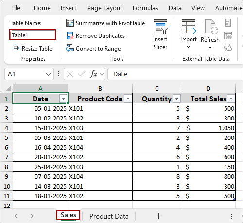
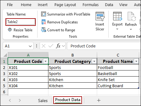
For this example, let’s assume you have two sheets: one named Sales with sales transaction data and another named Product Data with product details. Both sheets share a Product Code column.

Before you begin, make sure your data is formatted as an Excel Table. Here, we have the Sales sheet named Table1 and the Product Data sheet as Table2.

Now, let’s create the relationship between these two tables.

➤ Go to the Data tab on the ribbon.
➤ In the Data Tools group, click on Data Model and then Relationships.

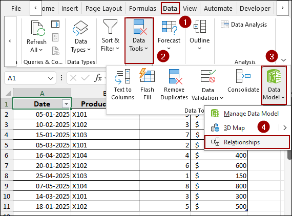
This will open the Manage Relationships window.

➤ Click New to create a new relationship.

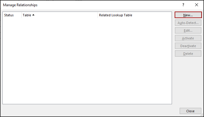
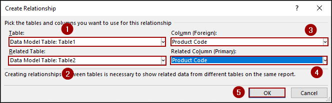
A Create Relationship dialog box will appear.

➤ In the Table dropdown, select Data Model Table: Table1.
➤ In the Related Table dropdown, select Data Model Table: Table2.
➤ In the Column (Foreign) dropdown, select Product Code.
➤ In the Related Column (Primary) dropdown, select Product Code.
➤ Click OK.

Thus, a link between the two sheets is created. Next, we will use this relationship to create a PivotTable.

➤ Go to the Insert tab on the ribbon.
➤ In the Tables group, click on PivotTable.
➤ From the dropdown, select From Data Model.

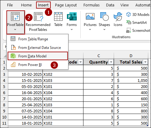
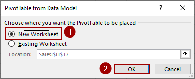
The PivotTable from Data Model window will open.

➤ Choose New Worksheet and click OK.

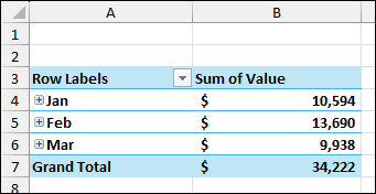
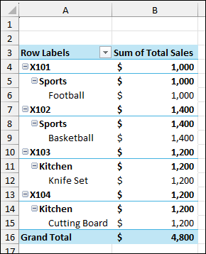
As a result, you will get a  PivotTable showing sales data for each product, with product categories from a separate sheet. This is a quick way to create Pivot Table from two sheets with the same column.

The PivotTable and PivotChart Wizard is a useful tool to create a Pivot Table combining data from multiple sheets, if the data has the exact same column headers. Here, we will use this tool to combine data ranges from multiple sheets and create a single Pivot Table.

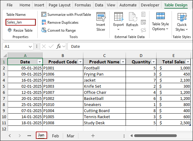
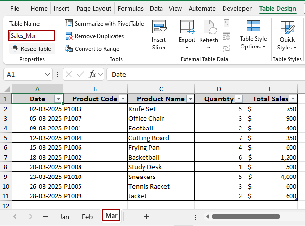
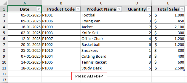
For this example, let’s assume we have three separate worksheets named Jan, Feb, and Mar, each with sales data.

➤ Press  Alt  +  D  +  P  on your keyboard to launch the “PivotTable and PivotChart Wizard” window.

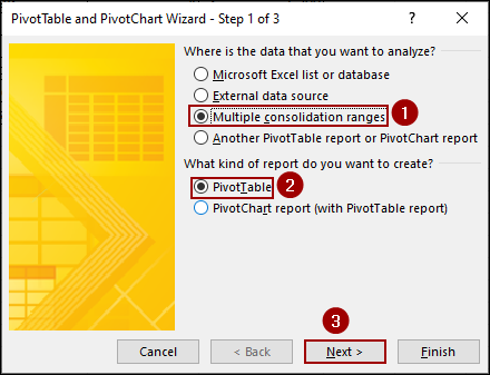
➤ Choose Multiple consolidation ranges and PivotTable to create a report.
➤ Click Next.

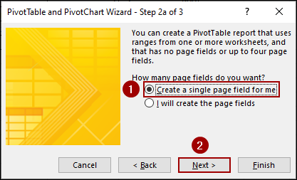
➤ Select Create a single page field for me to have Excel automatically create a field that distinguishes between your sheets.
➤ Click Next.

Now, you need to add the data ranges from each of your worksheets.

➤ Go to your first worksheet (e.g., Jan), select the data range (e.g., A1:E11), and click Add.

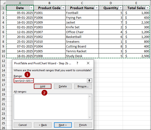
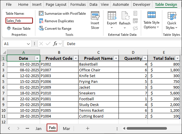
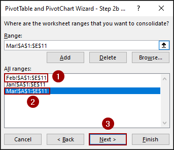
➤ Repeat this for each of your remaining worksheets (Feb and Mar).
➤ Click Next.

➤ Choose New worksheet option to place your PivotTable on a new sheet, then click Finish.

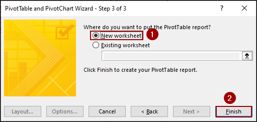
Excel will create a new sheet with a PivotTable, combining data from multiple sheets with the same columns.

The Append Queries feature from Power Query can easily combine data from multiple sheets with the same columns. This feature is helpful if you are working with a large dataset. Here, we will launch the Power Query Editor, use Append Queries to combine the data in a single query, and convert it into a Pivot Table.

For this example, we will use the same three sheets with sales data: Jan, Feb, and Mar.

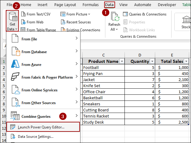
➤ Go to the Data tab.
➤ In the Get & Transform Data group, click Get Data.
➤ Select Launch Power Query Editor.

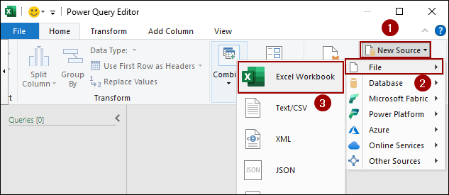
➤ From the Power Query Editor window, click New Source > File > Excel Workbook.

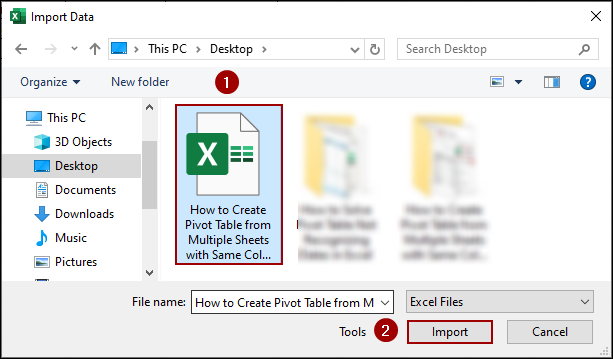
➤ In the file browser, locate and select your Excel file.
➤ Click Import.

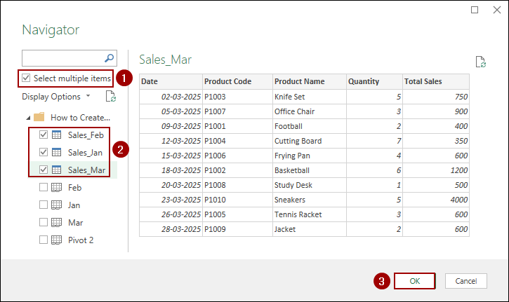
The Navigator window will appear.

➤ Checkmark the box for Select multiple items.
➤ Select your tables (Jan, Feb, and Mar).
➤ Click OK.

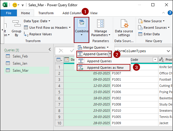
Thus, we will see a separate query for each of the sheets. Now, we need to append them.

➤ Go to the Home tab in the Power Query Editor.
➤ In the Combine group, click the dropdown menu and select Append Queries as New.

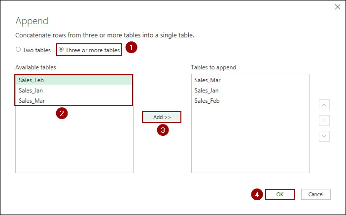
The Append dialog box will appear.

➤ Choose Three or more tables.
➤ Select all three tables (Sales_Jan, Sales_Feb, Sales_Mar) from the Available tables list and click Add.
➤ Click OK.

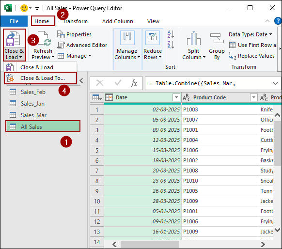
A new query named Append1 will be created, combining all data.

➤ Rename Append1 to a more descriptive name, like All Sales.
➤ On the Home tab, click Close & Load To.

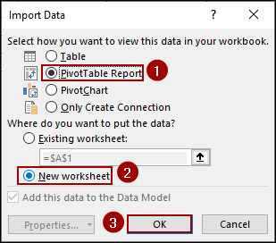
The Import Data dialog box will appear.

➤ Select PivotTable Report and New worksheet.
➤ Click OK.

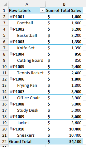
Finally, we will get a single Pivot Table, combining data from multiple sheets.

Frequently Asked Questions

Can I update the Pivot Table if I add new data to one of the sheets?

Yes, if you have built your Pivot Table using Power Query or the Data Model, simply refresh the query, and the Pivot Table will include the new data automatically.

Is there a limit to how many sheets I can combine for a Pivot Table?

There is no strict limit, but performance depends on your system. For large datasets, using Power Query with the Data Model is recommended to handle them efficiently.

What if my sheets are in different workbooks?

You can still combine them using Power Query, but you will need to connect each workbook as a data source and then append them before building your Pivot Table.

Concluding Words

Above, we have explored three effective ways to create a PivotTable from multiple sheets with the same column. While the PivotTable Wizard is a quick solution for simple tasks, the Data Model and Power Query‘s Append Queries feature offer more dynamic solutions for frequently updated data. If you have any queries, feel free to let us know in the comments section below.