How to Alternate Row Color Based on Group in Excel

When a column in your dataset has multiple common values in groups, highlighting every other common group allows you to better visualize your data. It enables users to quickly scan, compare, and analyze data.

To alternate row colors based on groups, you can use conditional formatting formulas with functions like IF, LEN, MOD, ISEVEN/ISODD, etc. While some formulas work directly, others require a helper column to assign numbers to the grouped values and highlight rows based on them.

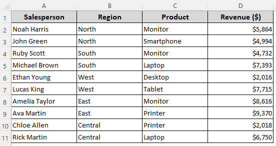
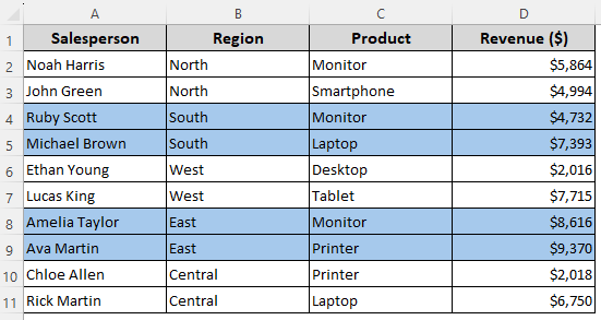
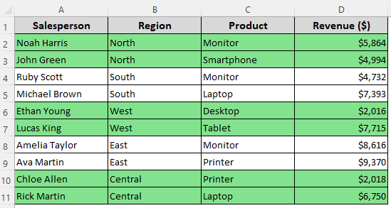
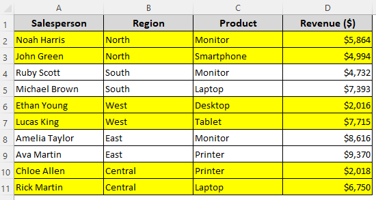
Our sample sales dataset has columns for Salesperson, Region, Product, and Revenue. In Column B, we have 5 grouped regions: North, South, West, East, and Central. Each group occupies 2 rows. Our goal is to highlight alternate rows based on the groups.

If each group in your dataset has the same number of rows, you can combine the ISEVEN, CEILING, and ROW functions to format every other group. For example, in our dataset, each region group takes 2 rows (North 2 rows, South 2 rows, etc.). To format such datasets based on groups, follow the steps given below:

➤ Select the range you want to highlight without the headers (A2:D11). Go to the Home tab and click on the Conditional Formatting drop-down. Choose New Rule from the menu to open the New Formatting Rule dialog box.

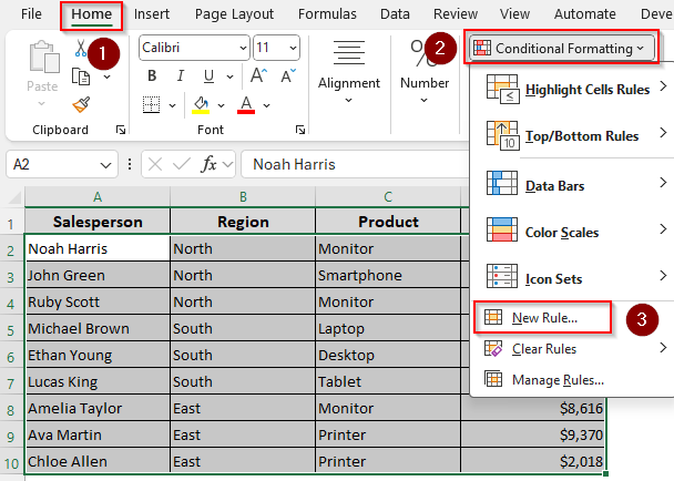
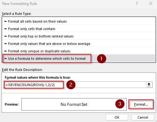
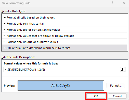
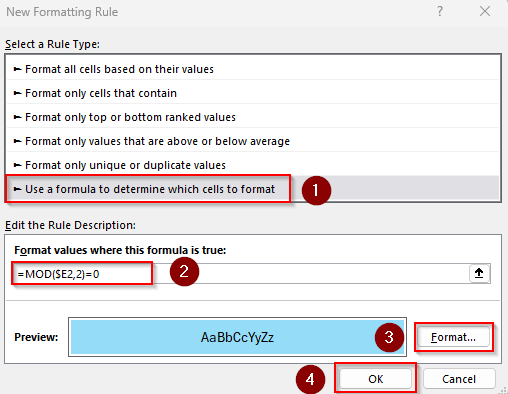
➤ From the Select a Rule Type group, click on Use a Formula to Determine Which Cells to Format.
➤ In the blank field under the Format Values Where This Formula Is True option, enter the following formula:

➤ As each of our groups takes 2 rows, we entered 2 in the formula. You need to replace 2 with your group size. For instance, if your groups have 3 rows each, use:

Similarly, for groups each taking 4 rows, use:

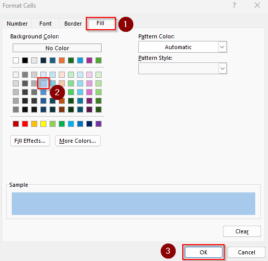
➤ After entering the appropriate formula, click on Format and use the Number, Font, Border, and Fill tabs to choose highlighting options. Click Ok when done.

➤ Close the New Formatting Rule dialog box by pressing Ok.

➤ Here’s the final output:

The previous method won’t work for variable group sizes. Therefore, we’ll use a different formula with the ISEVEN/ISODD and SUMPRODUCT functions that works for all group sizes. Below are the details:

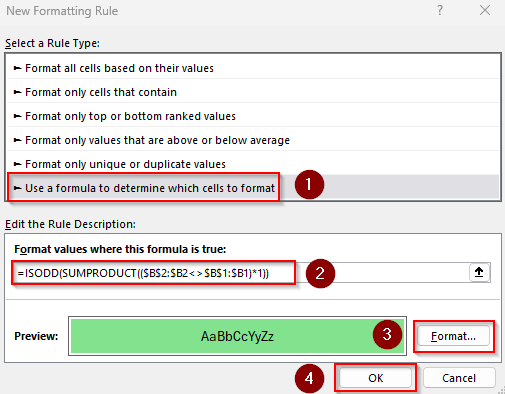
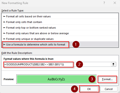
➤ Click and drag to highlight the cells you want to format (A2:D11), excluding the headers. Now, open the Home tab >> Conditional Formatting drop-down >> New Rule >> Use a Formula to Determine Which Cells to Format.
➤ Insert any of the following formulas in the Format Values Where This Formula Is True field:

To Start Formatting from the First Group

➤ Here, B1 and B2 are the first cells of the column containing the grouped values (including the header cell). You must change them to match your dataset while keeping the $ signs in place to lock the cells.
➤ Click on the Format option to choose a fill color to highlight and press Ok twice to close each window.

➤ Here’s the final result for ISODD:

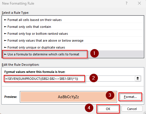
To Start Formatting from the Second Group

➤ Replace the cell references as needed. Set formatting rules and press Ok twice.

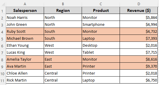
➤ Below is the output for ISEVEN:

Using the MOD and SUMPRODUCT functions, we can create a formula that checks every time a group changes. Based on this, Excel will apply conditional formatting rules in your specified range. Let’s get into the details:

➤ Start by selecting your dataset (A2:D11). From the Home tab >> Conditional Formatting drop-down >> New Rule >> Use a Formula to Determine Which Cells to Format.
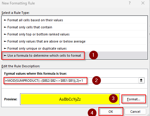
➤ Fill the formula box with the formula given below:

➤ Change B1 and B2 to the first and second cells of your group column.
➤ Apply highlighting rules using the Format button. Press Ok.

➤ Click Ok again to see the formatted cells.

A helper column allows you to assign a common number to each row of a group. Depending on these numbers assigned to each group, we can use a formula with the MOD function to highlight alternating rows. Here’s how:

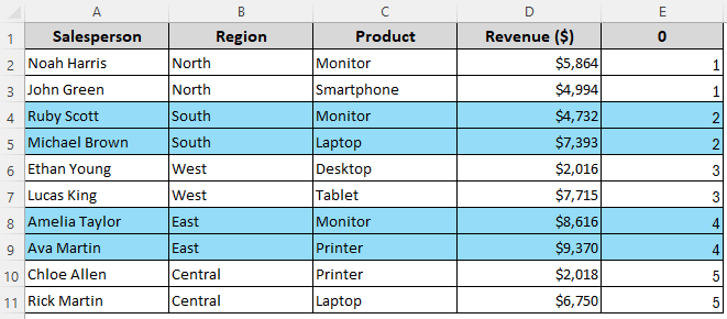
➤ Insert a helper column (Column E) and set 0 as its header. You can also keep the header row empty. However, any other texts or numbers will cause an error.
➤ Enter this formula in its first cell (E2):

➤ Replace the first and second cells of the group column B1 and B2, along with the first cell of the helper column E1, according to your dataset.
➤ Click Enter and drag the formula down to fill the remaining cells. Excel will assign the appropriate numbers to the relevant groups. This formula increments the group number whenever the Region changes.

➤ Now, select your data range with the helper column (A2:E11) and go to the Home tab >> Conditional Formatting drop-down >> New Rule >> Use a Formula to Determine Which Cells to Format.
➤ In the formula box, type the following formula to highlight the groups associated with even numbers:

➤ Set the formatting rules using the Format button and press Ok.

➤ Click Ok to close the window and review the result.

Similar to the previous method, we can generate numbers in a helper column with a formula. After that, we can use the ISEVEN or ISODD function to highlight rows corresponding to their assigned even or odd numbers. Here are the details:

➤ Select the header cell of the helper column (E1) and enter 0.
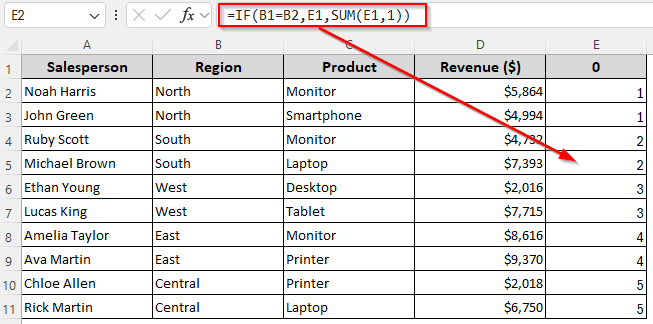
➤ In the following cell (E2), insert this formula:

➤ Replace B1 and B2 with the first two cells of your header column and change E1 to the first cell of the helper column.
➤ Press Enter and drag the formula down to autofill the following cells.

➤ Choose your data range including the helper column (A2:E11). Click on the Home tab >> Conditional Formatting drop-down >> New Rule >> Use a Formula to Determine Which Cells to Format.
➤ In the formula box, enter any of the formulas given below:

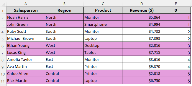
Highlight Rows with Odd Numbers

➤ Here, $E2 is the first cell of the helper column excluding the header. Change it as needed.
➤ Set formatting rules.

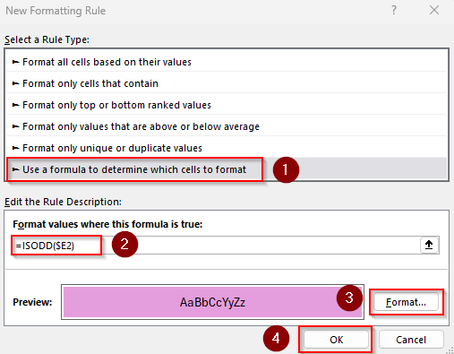
➤ Press Ok twice and check the output.

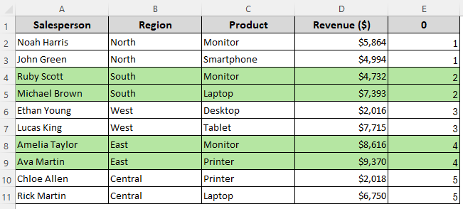
Highlight Rows with Even Numbers

➤ Replace $E2 as required.
➤ Apply formatting styles.

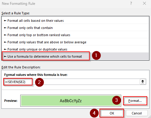
➤ Click Ok twice and review the result:

Frequently Asked Questions

How to get every other row a different color in Excel?

First, select your entire data range (A2:D11) and go to the Home tab >> Conditional Formatting drop-down >> New Rule >> Use a Formula to Determine Which Cells to Format. In the formula box, enter:

=ISEVEN(ROW()) or, =ISODD(ROW())

Apply formatting rules and press Ok twice to color every other row automatically.

How to remove highlighting from alternate rows?

To remove highlighting rules applied with conditional formatting, select the highlighted data range, go to the Home tab and click on the Conditional Formatting drop-down. Choose Manage Rules, select the rule you want to remove, and press Delete.

How do I maintain alternate row coloring when I add new rows?

To make alternate row colors automatically adjust when you add or delete rows, you need to convert your dataset into an Excel Table and enable Banded Rows. For this, select any cell in your dataset and press  Ctrl  +  T . In the dialog box, make sure the range is correct and check My table Has Headers if your data has headers. Click Ok. Now, open the Table Design tab. In the Table Style Options group, check the box Banded Rows.

Concluding Words

For a direct approach, you can highlight based on a single formula. When you use a helper column, you can hide the column later for a cleaner look. However, if your rule depends on a helper column and you delete that column afterward, Excel will lose the reference (#REF!) and the highlighting will break. Finally, make sure you use the $ signs as given in the formulas to get accurate results.