The QUERY function is one of the most versatile functions in Google Sheets. It allows you to perform tasks like filtering, sorting, grouping, and summarizing, using a language very similar to SQL (Structured Query Language). With QUERY function, you can transform a raw dataset into a filtered and aggregated report with a single formula. In this article, we will learn about all the aspects of QUERY functions in Google Sheets.
Syntax of QUERY Function in Google Sheets
Before diving into the complex operations, let’s learn about the basic structure of the QUERY function. Here, we will cover the fundamental components needed to construct any QUERY formula.
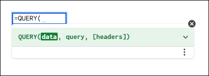
The function takes three arguments.
➤ data: This is the range of cells you want to query, such as A1:F11.
➤ query: This is the SQL-like command, enclosed in quotation marks, that specifies what you want the function to do (e.g., select, where, group by).
➤ [headers]: This optional number tells the function how many header rows are present at the top of your data.
Applying QUERY Function to Filter Data Using Conditions
One of the most common uses for the QUERY function is to filter a large dataset based on specific conditions.
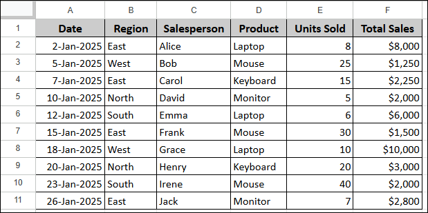
Suppose we have a sample dataset containing Date, Region, Salesperson, Product, Units Sold, and Total Sales. In this section, we will use the where clause to pull out specific subsets of data.
Single Condition
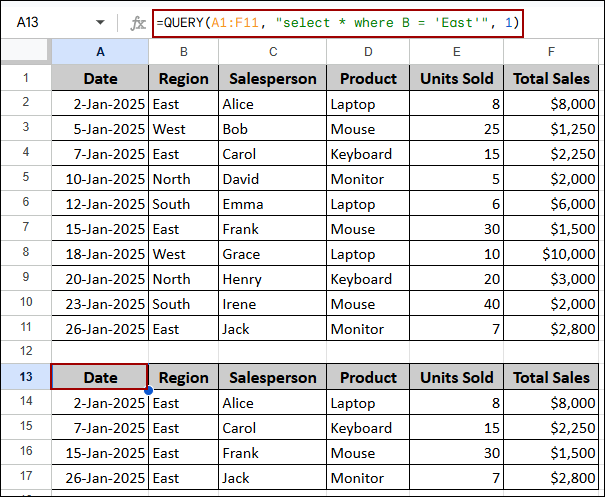
To filter data, we will use the where clause in the query string. Here, we will filter the sales data to show only entries where the Region is ‘East’.
➤ Choose a cell A13, write down the formula below, and press ENTER.
=QUERY(A1:F11, "select * where B = 'East'", 1)
Formula Breakdown:
- A1:F11: The range containing the data.
- “select *”: Selects all columns (*).
- “where B = ‘East'”: Filters the selected data to include only rows where Column B (Region) is exactly ‘East’.
As a result, we will get all sales records where the region is East.
Multiple Criteria (AND and OR)
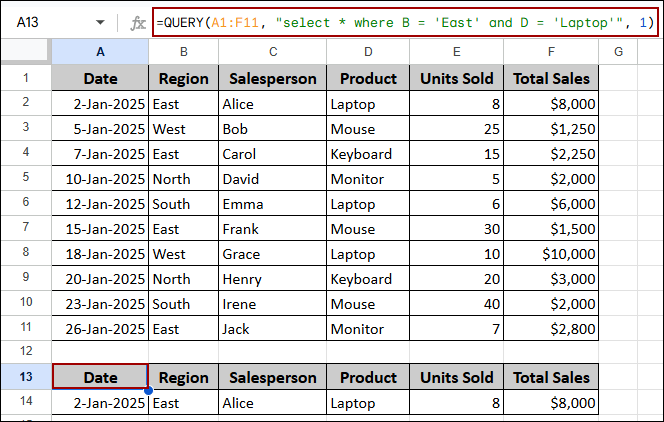
You can use logical operators like AND and OR to apply multiple conditions inside the QUERY function. Using the AND operator, we will filter the data to find all sales in the ‘East’ region and where the Product is ‘Laptop’, requiring both conditions to be met.
➤ Select cell A13, write down the formula below, and press ENTER.
=QUERY(A1:F11, "select * where B = 'East' and D = 'Laptop'", 1)
Formula Breakdown:
- A1:F11: The range containing the data.
- “select *”: Selects all columns (*).
- “where B = ‘East’ and D = ‘Laptop'”: Filters the data to include rows where Column B is ‘East’ AND Column D is ‘Laptop’.
The output returns a single row. This row is the only record that satisfies both criteria: the Region is East and the Product is Laptop.
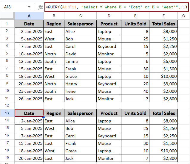
To find sales that meet at least one of two conditions, we will use the OR operator to identify all sales from either the ‘East’ region or the ‘West’ region.
➤ Select cell A13, put the formula below, and hit ENTER.
=QUERY(A1:F11, "select * where B = 'East' or B = 'West'", 1)
Formula Breakdown:
- A1:F11: The input data.
- “select *”: Retrieves all columns from the dataset.
- “where B = ‘East’ or B = ‘West'”: Filters the data to include rows where Column B is either ‘East’ OR Column B is ‘West’.
The result shows a consolidated list of 6 records, which includes all transactions from the East region and all transactions from the West region.
Excluding Data
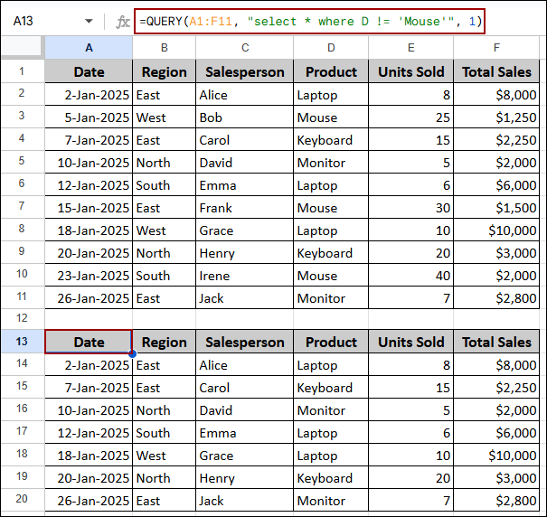
If you need to exclude certain data points, you can use the not equals(!=) operator. In this example, we will exclude all transactions where the Product is ‘Mouse’ from the final report.
➤ Choose a cell A13, put the formula below, and click ENTER.
=QUERY(A1:F11, "select * where D != 'Mouse'", 1)
Formula Breakdown:
- A1:F11: The source data.
- “select *”: Selects all available columns.
- “where D != ‘Mouse'”: Applies a negation filter, ensuring rows where Column D (Product) is NOT ‘Mouse’ are returned.
Thus, all transactions involving the Product ‘Mouse’ have been successfully removed from the output.
Sorting and Ordering Data
The order by clause in the QUERY function is used to sort the resulting data. In this section, we will demonstrate how to rearrange data based on single columns, multiple columns, and date/value order.
Using Order By Clause for Sorting Single Column
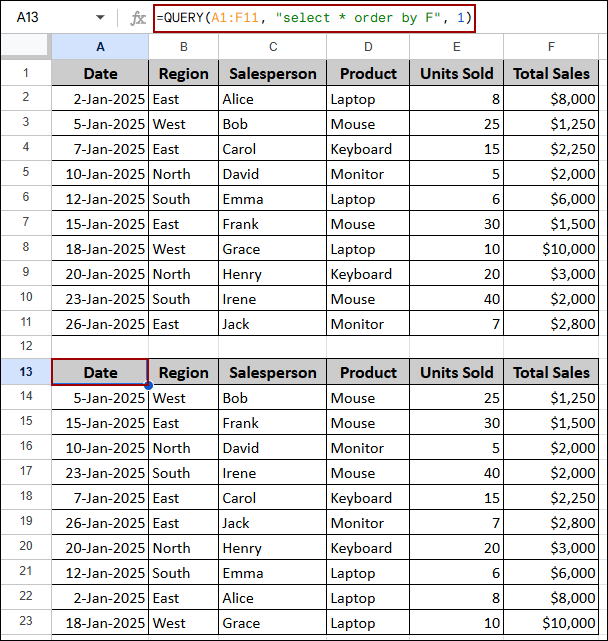
To arrange the data sequentially by transaction value, we will sort the data by the Total Sales column (Column F) in ascending order (smallest to largest).
➤ Choose a cell A13, type the formula below, and press ENTER.
=QUERY(A1:F11, "select * order by F", 1)
Formula Breakdown:
- A1:F11: The range containing your data.
- “select *”: Retrieves all columns.
- “order by F”: Sorts the selected data based on Column F (Total Sales) using the default ascending order.
The table is now sorted by the Total Sales column, starting with the lowest value and ending with the highest value.
Sorting by Multiple Columns
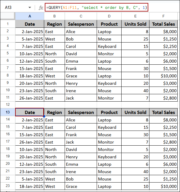
You can also use the QUERY function in Google Sheets to sort data by multiple columns. Here, we will sort the output first by Region (Column B) and then refine the order by Salesperson (Column C).
➤ Choose a cell A13, write down the formula below, and press ENTER.
=QUERY(A1:F11, "select * order by B, C", 1)
Formula Breakdown:
- A1:F11: The input data source.
- “select *”: Returns all fields.
- “order by B, C”: Sorts the data primarily by Column B (Region) and secondarily by Column C (Salesperson).
The data is now grouped by Region. Within each region, the Salespeople are sorted alphabetically.
Sorting in Descending Order
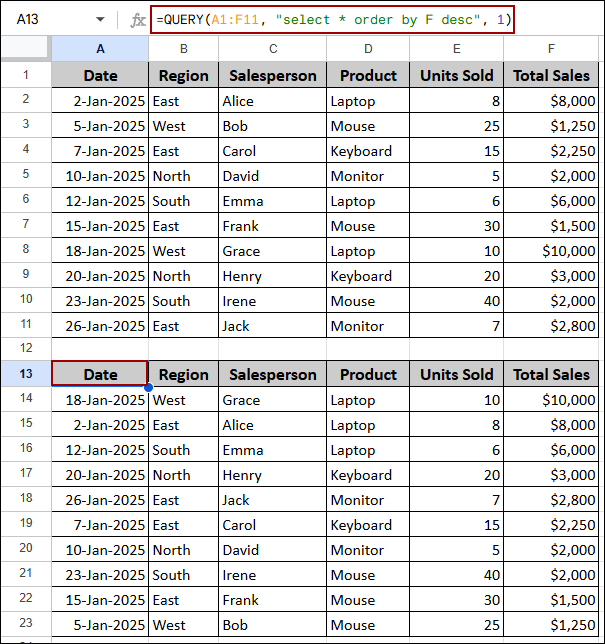
To view data from largest to smallest, we can specify the desc operator in the QUERY string. In this part, we will sort the Total Sales (Column F) in descending order to immediately see the highest-value transactions at the top.
➤ Choose a cell A13, write down the formula below, and press ENTER.
=QUERY(A1:F11, "select * order by F desc", 1)
Formula Breakdown:
- A1:F11: The range under query.
- “select *”: Retrieves all columns.
- “order by F desc”: Sorts the data by Column F, forcing the sort order to be descending (largest to smallest).
The highest sales figures now appear at the top, starting with the highest value and descending to the lowest sale.
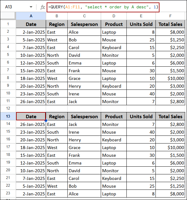
Sorting by Date
To easily track recent activity, we will sort the data using the Date column (Column A) in descending order, showing the most recent transactions first.
➤ Select cell A13, type the formula below, and hit ENTER.
=QUERY(A1:F11, "select * order by A desc", 1)
Formula Breakdown:
- A1:F11: The range containing your data.
- “select *”: Returns all columns.
- “order by A desc”: Sorts the data based on Column A (Date) in descending order.
The data is sorted with the latest dates appearing first and the oldest dates appearing last.
Grouping and Summarizing Data
You use the group by clause to group data along with aggregation functions like SUM, COUNT, AVG, MIN, or MAX. Using these functions inside the QUERY string, you will be able to group and summarize data according to your choice.
Using Group By Clause for Sorting Single Column
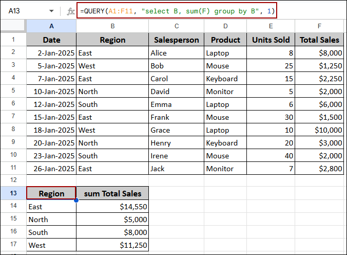
Here, we will calculate the Total Sales for each unique Region using SUM(F) and group the results by Column B.
➤ Select cell A13, put the formula below, and click ENTER.
=QUERY(A1:F11, "select B, sum(F) group by B", 1)
Formula Breakdown:
- A1:F11: The source data range.
- “select B, sum(F)”: Selects the Region (B) and performs a summation on the Total Sales (F).
- “group by B”: Instructs the query to consolidate the rows based on the unique values in Column B.
This formula returns a summarized table showing the sum of all sales for each unique Region.
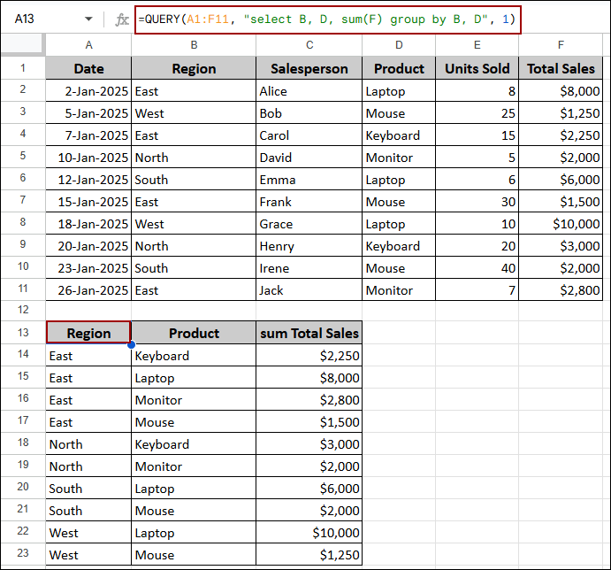
Grouping by Multiple Columns
Similarly, using the QUERY function, we will calculate Total Sales broken down by both Region and Product. Then, we will group both Column B and Column D with a single formula. It means we’re applying QUERY function here to group by multiple columns.
➤ Choose a cell A13, write down the formula below, and press ENTER.
=QUERY(A1:F11, "select B, D, sum(F) group by B, D", 1)
Formula Breakdown:
- A1:F11: The input data.
- “select B, D, sum(F)”: Selects Region (B), Product (D), and the sum of Total Sales (F).
- “group by B, D”: Groups the results based on the unique pairing of values from Column B and Column D.
The output shows the Total Sales for every unique combination of Region and Product.
Summing with Group By
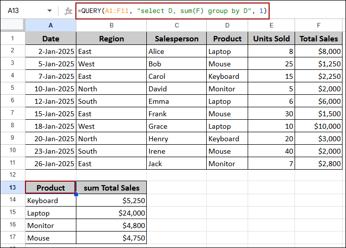
Suppose you need to identify the top revenue from a list. You can use the QUERY function in Google Sheets to summarize the Total Sales (Column F) by grouping the results according to Product (Column D).
➤ Select cell A13, type the formula below, and click ENTER.
=QUERY(A1:F11, "select D, sum(F) group by D", 1)
Formula Breakdown:
- A1:F11: The data range.
- “select D, sum(F)”: Retrieves the Product (D) and the aggregated sum of Total Sales (F).
- “group by D”: Consolidates the data rows by each unique value found in Column D.
As a result, the table summarizes the total revenue generated by each of the four unique product types in the dataset.
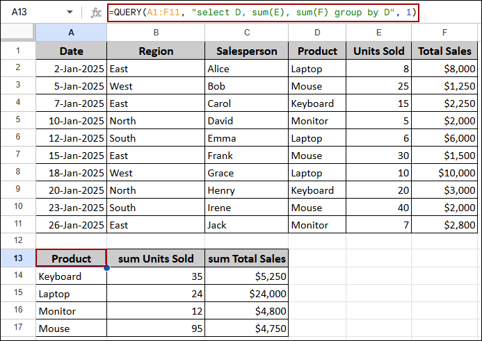
Summing Multiple Columns
To get a complete summary, we will aggregate both the sum of Units Sold (Column E) and the sum of Total Sales (Column F), grouped by Product (Column D).
➤ Similarly, choose a cell A13, put the formula in the cell, and apply the formula by pressing ENTER.
=QUERY(A1:F11, "select D, sum(E), sum(F) group by D", 1)
Formula Breakdown:
- A1:F11: The source data.
- “select D, sum(E), sum(F)”: Selects the Product (D) and aggregates the sums of both Column E and Column F.
- “group by D”: Organizes the summarized data by Column D.
Finally, the result provides a dual summary for each product, showing both the total quantity sold (sum Units Sold) and the total revenue generated (sum Total Sales).
Utilizing QUERY Function to Count Data
The COUNT function in the QUERY string is used for summarizing data by counting specific data. Here, we will learn how to count the number of rows and unique values with specific criteria.
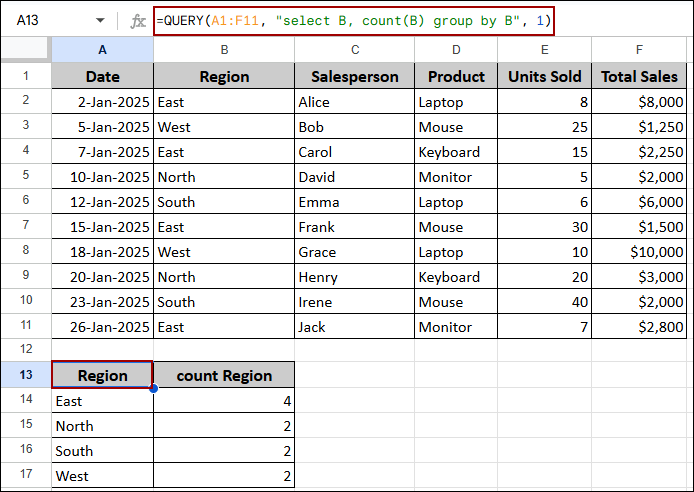
Counting Rows
In this part, we will count the number of transactions per region using the COUNT function and then group the results using the group by clause in the QUERY string.
➤ Choose a cell A13, write down the formula below, and press ENTER.
=QUERY(A1:F11, "select B, count(B) group by B", 1)
Formula Breakdown:
- A1:F11: The range containing your data.
- “select B, count(B)”: Selects the Region (B) and computes the count of records in Column B.
- “group by B”: Consolidates the counts based on the unique values in Column B.
Finally, the summary table shows the number of transactions that occurred in each Region.
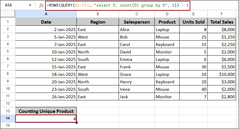
Counting Unique Values
Similarly, we will count the number of unique products in the dataset by nesting the QUERY function that groups the products inside a ROWS function.
➤ Select cell A14, put the formula below, and click ENTER.
=ROWS(QUERY(A1:F11, "select D, count(D) group by D", 1)) - 1
Formula Breakdown:
- QUERY(A1:F11, “select D, count(D) group by D”, 1): Generates a table with one row for each unique Product.
- ROWS(…): Counts the total number of rows (including the header) in the interim table.
- – 1: Subtracts 1 to remove the header row, yielding the final count of unique products.
The final calculated value in the cell is 4, which accurately represents the total number of unique product types in the data range.
Query Function for Dates with Proper Format
When querying data based on a date, the QUERY function requires the date to be enclosed within the date keyword and single quotes, following the format YYYY-MM-DD. Here, we will demonstrate the required format to successfully filter data by date.
Problem:
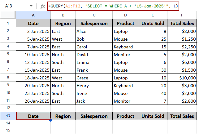
Suppose we want to select all sales with a Date (Column A) after January 15, 2025.
➤ Start by choosing a cell A13, writing the formula, and hitting ENTER.
=QUERY(A1:F12, "SELECT * WHERE A > '15-Jan-2025'", 1)
The query returns no results because the date string was not correctly recognized by the QUERY function.
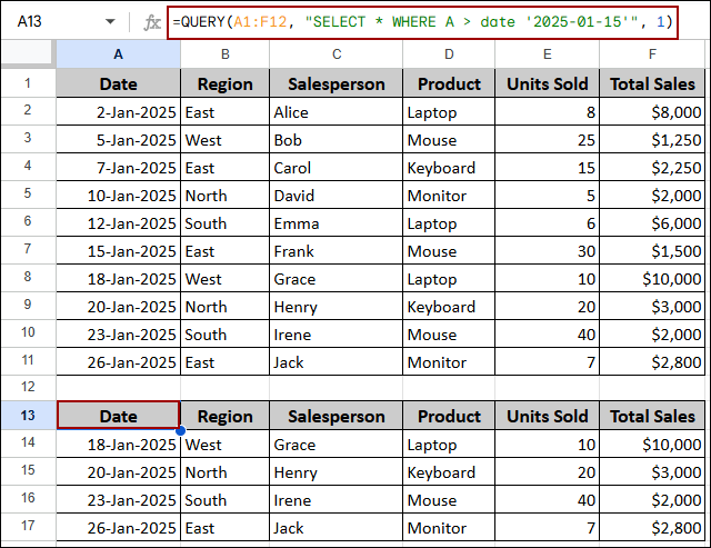
Solution:
You need to use the required date keyword and the YYYY-MM-DD format to successfully filter the data.
➤ In cell A13, write down the formula below, and click ENTER.
=QUERY(A1:F12, "SELECT * WHERE A > date '2025-01-15'", 1)
Formula Breakdown:
- A1:F12: The range under evaluation.
- “SELECT * WHERE A > date ‘2025-01-15′”: Filters the data to include rows where Column A (Date) is strictly greater than the specified date, using the mandatory date ‘YYYY-MM-DD‘ structure.
Finally, the QUERY function filters the data, returning the 4 transactions that occurred after January 15, 2025.
Querying Data from Multiple Sources
The QUERY function can also combine data with criteria from non-adjacent ranges or even different sheets within the same formula. In this part, we will see how to use curly braces {} to combine data from different sheets and non-adjacent cells.
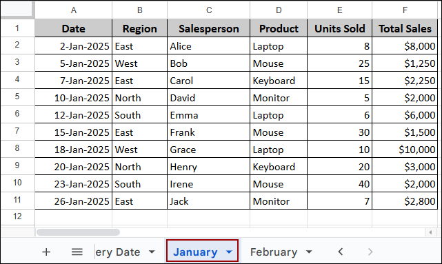
Querying from Multiple Sheets
Suppose we have a sales transaction for January in a sheet named January.
In another sheet named February, we have the sales record for February.
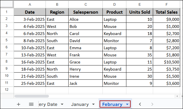
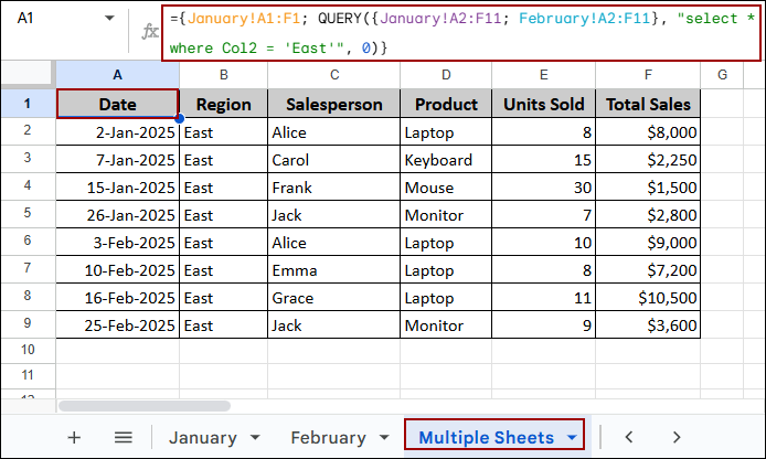
To consolidate the monthly data, we will combine the records from both sheets and then filter the dataset to show only the ‘East’ region.
➤ In a new sheet, choose a cell (A13), write down the formula below, and press ENTER.
={ 'January'!A1:F1; QUERY({'January'!A2:F11; 'February'!A2:F11}, "select * where Col2 = 'East'", 0) }
Formula Breakdown:
- {…}: The curly braces combine all specified ranges into a single, temporary virtual array. The header row A1:F1 is manually added first.
- {‘January’!A2:F11; ‘February’!A2:F11}: Vertically stacks the data rows (;) from the two separate sheets.
- “select * where Col2 = ‘East'”: Filters the combined data. Since the ranges were merged, columns are referenced numerically (Col1, Col2, etc.); Col2 represents the Region column.
- 0: Specifies zero header rows for the inner QUERY to prevent the function from double-counting the headers.
The resulting table combines the records from the January and February sheets and filters them to show only transactions from the East region.
Combining Non-adjacent Ranges
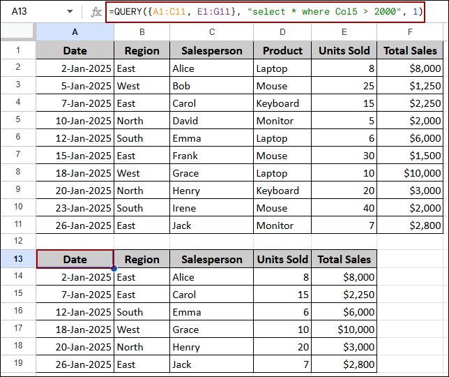
You can use the QUERY function to combine non-adjacent ranges with specific criteria with a single formula. Here, we will combine non-adjacent columns (A, B, C, and E, F), filtering for sales greater than $2,000.
➤ Choose any cell (A13), write down the formula below, and press ENTER.
=QUERY({A1:C11, E1:F11}, "select * where Col5 > 2000", 1)
Formula Breakdown:
- {A1:C11, E1:F11}: Combines the selected ranges horizontally (side-by-side) using the comma ,. This forms a virtual table with 5 columns.
- “select * where Col5 > 2000”: Filters the data in the virtual table where the fifth column (Col5, which holds the Total Sales value from original column F) is greater than 2000.
The result selects only the specified columns and filters the records to show only those where Total Sales exceeds $2,000.
Formatting and Customizing Output
The QUERY function can clean data and make it more readable when summarizing data. In this section, we will see how to create pivot tables and assign clear labels to aggregated results.
Creating Pivot Table Using QUERY Function
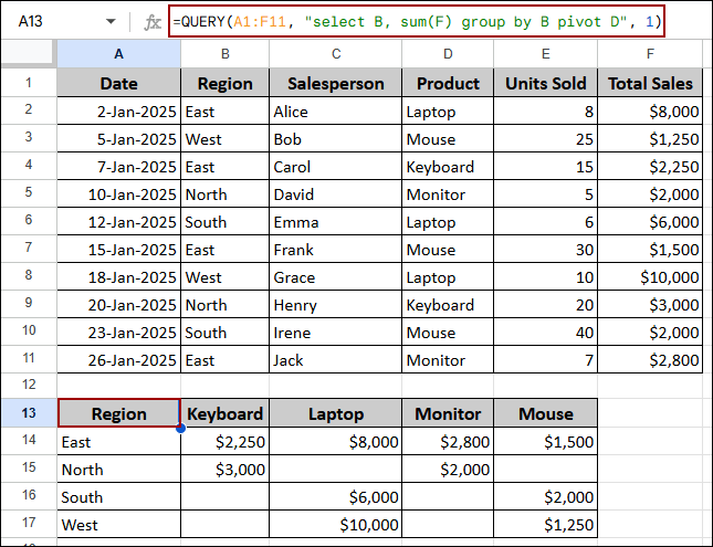
The pivot clause in the QUERY string is used to summarize data by transposing and combining. Here, we will calculate the Total Sales (sum of F) grouped by Region (B), and pivot the unique Product (D) values into separate columns, effectively creating a pivot table.
➤ Choose a cell A13, write down the formula below, and press ENTER.
=QUERY(A1:F11, "select B, sum(F) group by B pivot D", 1)
Formula Breakdown:
- A1:F11: The range containing the source data.
- “select B, sum(F) group by B”: Establishes the primary aggregation (Region and Total Sales).
- “pivot D”: Restructures the output so that the unique values from Column D (Product) become new column headers, organizing the sum(F) data beneath them.
This formula creates a pivot table where Regions are rows and Products are column headers.
Adding Labels to Columns
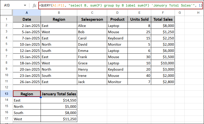
Utilizing the QUERY function, you can also add custom labels in Google Sheets. Here, we will calculate the Total Sales per Region and then rename the automatically generated column header (sum Total Sales) to a clearer name, ‘January Total Sales’, using the label clause.
➤ In a cell (A13), write down the formula below, and press ENTER.
=QUERY(A1:F11, "select B, sum(F) group by B label sum(F) 'January Total Sales'", 1)
Formula Breakdown:
- A1:F11: The data source.
- “select B, sum(F) group by B”: Sets up the regional summary.
- “label sum(F) ‘January Total Sales'”: Customizes the header of the sum(F) column to the desired text.
The resulting summarized table is identical to the basic group by result, but the second column’s header has been replaced with the custom, reader-friendly label: ‘January Total Sales’.
Frequently Asked Questions
Why do I sometimes have to use Col1, Col2, etc.?
When you combine ranges with curly braces {}, you must refer to columns numerically, regardless of their original sheet letter.
Why did my header rows disappear after applying the formula?
Check the third argument in the formula; it should be 1 if your data includes one header row. If it’s 0, the headers will be excluded.
How do I filter for a specific text value?
Use the where clause with the column and the text enclosed in single quotes, such as “where C = ‘Alice'”.
Concluding Words
Above, we have covered all features of the QUERY function in Google Sheets. This function is more advanced than others as it can provide all types of solutions like sorting, filtering, summarizing, anf grouping. By utilizing the SQL clauses where, order by, group by, and pivot, you can transform raw datasets into dynamic and automatically updating reports. Using curly braces {} in the string provides data collection from multiple sheets. If you have any questions, feel free to drop them in the comment section below.