Data validation is a built-in tool in Google Sheets that can help you stop problems even before they start. You can use it to set rules on what data can or cannot be entered into a cell. Data validation makes it simple to instruct users and reduce errors. Whether you’re entering a custom formula to verify that an email address is valid, limiting entries to integers only, or creating a drop-down list of job statuses, it’s easy to do using data validation.
What Is Data Validation in Google Sheets?
Google Sheets has a feature called data validation that restricts the type of data entered into a cell or range. It’s useful for spreadsheets, databases and forms for which clean data is important. It is useful to:

- Prevent interruptions to errors and misinformation.
- Create drop-down menus so selection is easy.
- Limit your data to specific types (text, dates and numbers).
Data Validation in Google Sheets Using Custom Formula
When standard validation isn’t enough, you can construct strong, adaptable criteria for cell inputs using Google Sheets’ Custom Formula option for data validation. Let’s look at the dataset below to determine whether to show a warning or reject invalid input in column D.
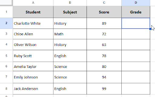
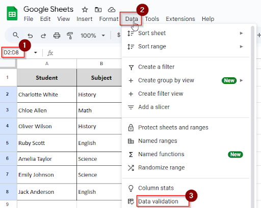
➤ Select the cell range D2:D8
➤ Go to Data > Data validation.
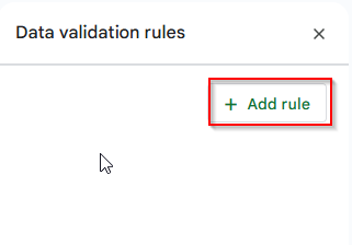
➤ Click on the” Add rule” option.
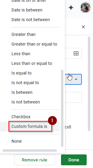
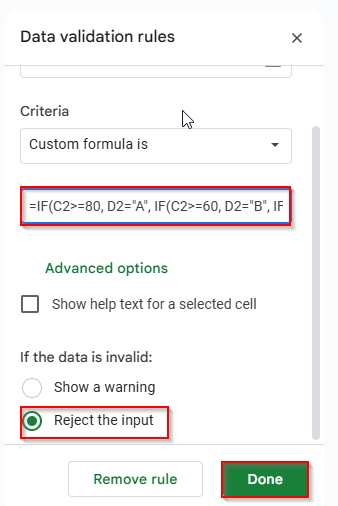
➤ Under Criteria, choose “Custom formula is”.
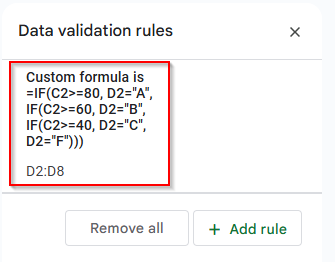
➤ Enter the following formula:
➤ Select Reject input
➤ Click Done
➤ Now you can see the data validation rules in your selected cell range.
➤ Enter the input in column D.
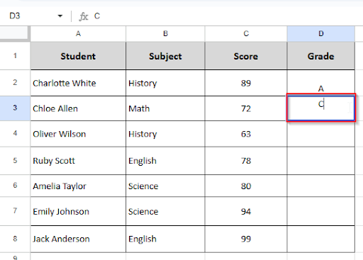
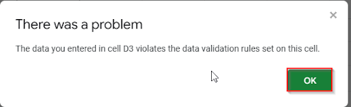
➤ When you enter the wrong input, it will show a message and reject that input.
Data Validation Based on Another Cell in Google Sheets
Sometimes, one cell’s input must depend on another’s value. Data validation is helpful when you want various dropdown options based on which category is selected, or you might want to only let a user select from a list if another column contains a particular value. Let’s follow the steps below to get the whole idea of data validation based on another cell in Google Sheets:
➤ In Sheet 2, Select A2:A4
➤ Click Data > Named ranges
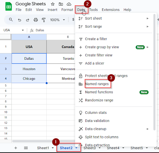
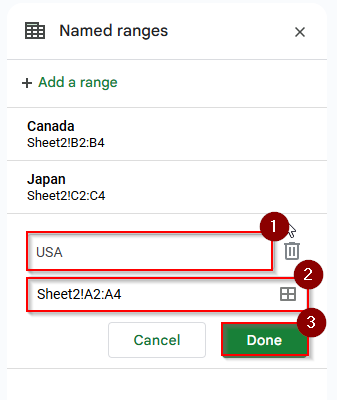
➤ Name the range: USA
➤ Click Done
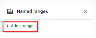
➤ Click the Add a range option.
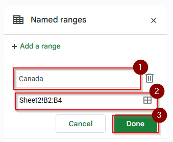
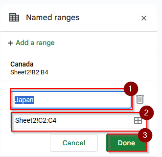
➤ Select the range B2:B4 and name it “Canada”
➤ Click Done.
➤ Select the range C2:C4 and name it “Japan”
➤ Click Done.
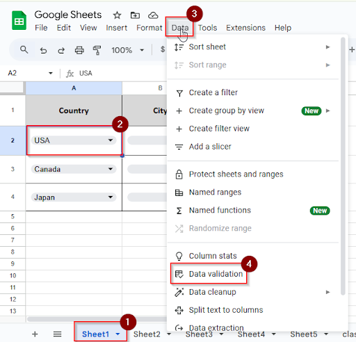
➤ In Sheet 1, click on the cell A2
➤ Click Data > Data validation
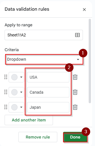
➤ Under Criteria, select Dropdown
➤ Add these options: USA, Canada, Japan
➤ Click Done
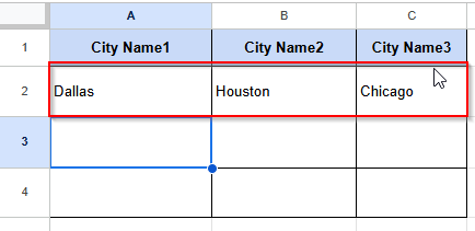
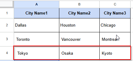
➤ Create another sheet and name it “sheet3”.
➤ Click on cell A2 and type this formula:
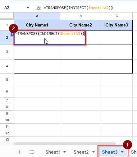
➤ Press Enter and see the result. All the city names in the USA are listed.
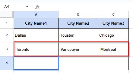
➤ Click on cell A3 and type this formula
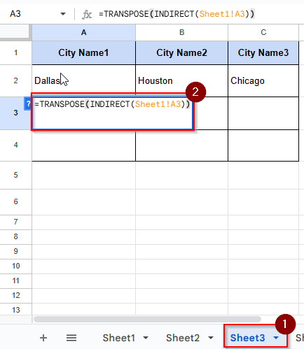
➤ Press Enter and see the result. All the city names of Canada are listed.
➤ Click on cell A4 and type this formula:
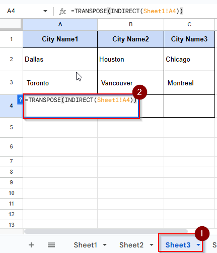
➤ Press Enter and see the result. All the city names of Japan are listed.
➤ Back to Sheet 1 and click on cell B2
➤ Click Data > Data validation
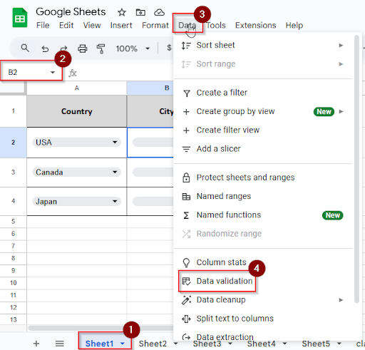
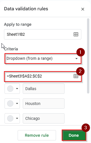
➤ Under Criteria, choose: “Dropdown from range”
➤ Set the range to: Sheet3!A2:C2
➤ Click Done.
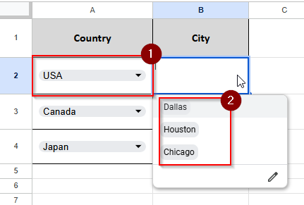
➤ Now see the result in Sheet 1. When you select the country name USA from the dropdown menu, it will show the city names of USA in column B2.
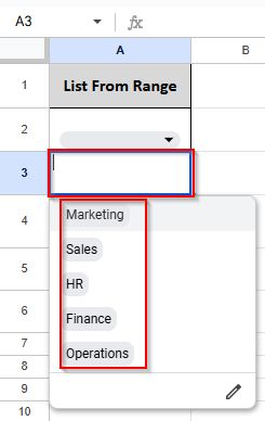
Data Validation List from a Range Formula in Google Sheets
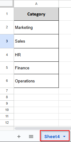
You can pull the dropdown items from a dynamic list, which is useful for managing a team, keeping track of inventory, and creating forms. When your data changes, your dropdown menu can adapt or expand automatically. Let’s look at the dataset below, where you have a department category in Sheet 4. To appear on this list as a dropdown in sheet 5, what you have to do is:
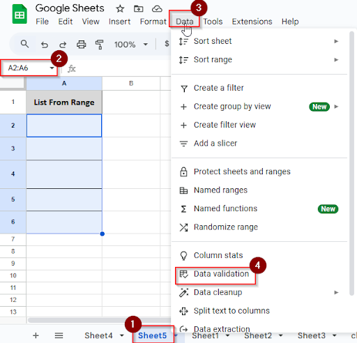
➤ Select the cell range A2:A6 on Sheet5
➤ Click on Data > Data validation
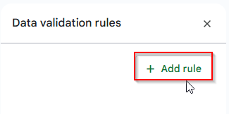
➤ Click the “Add rule” option.
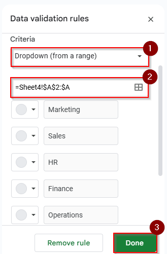
➤ Under Criteria, choose: Dropdown from a range
➤ In the range section, type this range: Sheet4!A2:A
➤ Click Done
Now you can see the result. You can choose any option from the dropdown list range on your selected cell range.
Frequently Asked Questions
What’s the difference between “Dropdown” and “Dropdown from a range”?
A Dropdown is manually typed with a list of options, but a dropdown from a range pulls items from cells anywhere in your sheet.
How can I use data validation to limit dates or numbers?
At first, under the validation criteria, select a number or date. Next, set the rules, such as greater than, between, or before today.
What happens if incorrect data is entered?
When a user enters incorrect data, you have the option to display a warning (the data remains, but is marked) and reject the input because data that doesn’t comply with the regulation won’t be accepted.
Concluding Words
Data validation can improve your spreadsheet management in Google Sheets. Whether you’re extracting options from a dynamic range or producing dropdowns from a fixed list, these techniques can help you save time and make clean data.