Conditional formatting is an effective Excel feature that visually enhances your data by applying color or style changes based on specific conditions. When combined with checkboxes, it becomes an interactive tool for tracking progress, managing tasks, or highlighting completed items. For example, you can use it to turn rows green when a task is marked complete, or gray when a checkbox is unchecked which gives your sheet a professional and dynamic look.
In this article, you’ll learn how to apply conditional formatting to checkboxes in Excel using simple step-by-step methods. We’ll cover both manual and VBA-based approaches to help you control your formatting efficiently, even for large datasets. Let’s get started.
Steps to apply conditional formatting to checkboxes in Excel:
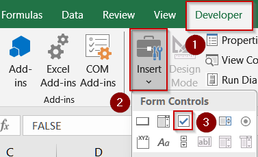
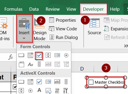
➤ Insert a checkbox in column C using the Developer tab >> Insert option >> Form Controls >> Checkbox.
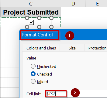
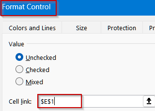
➤ Right-click the checkbox and select Format Control.
➤ In the Cell link box, select the cell where the checkbox state will be stored (e.g., C2) and click OK.
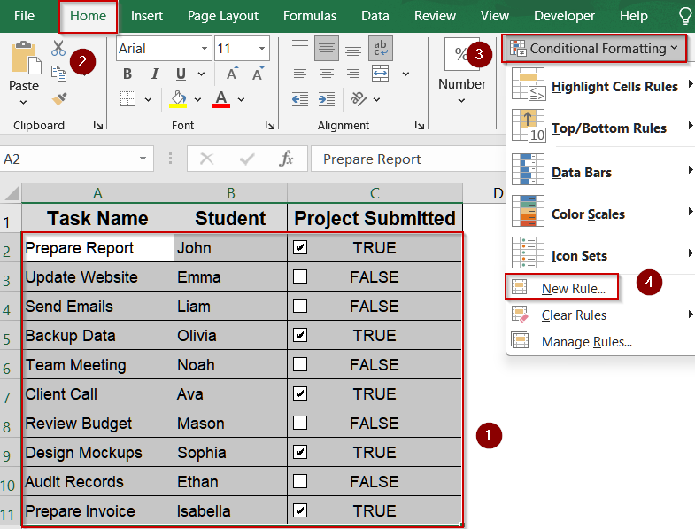
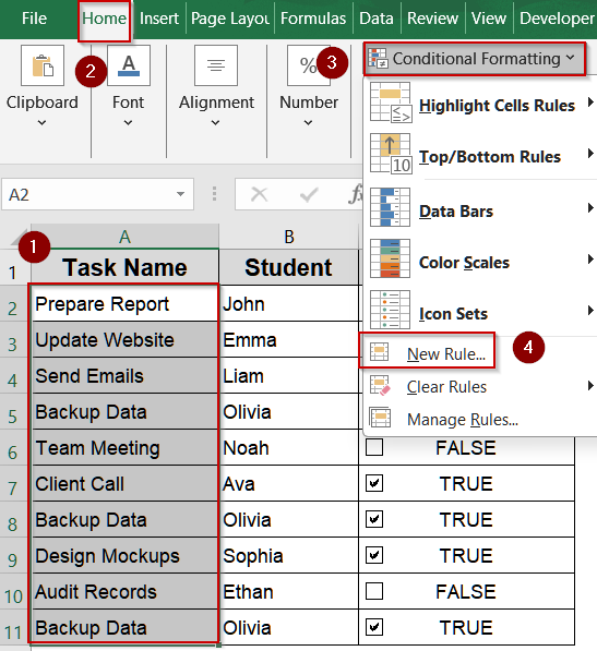
➤ Select the range of rows or cells you want to format (e.g., A2:C11).
➤ Go to Home >> Conditional Formatting >> New Rule.
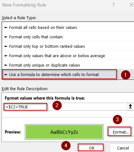
➤ Choose Use a formula to determine which cells to format.
➤ Enter the formula: =$C2=TRUE
➤ Click Format, select a fill color (e.g., green) to highlight completed tasks, then click OK twice.

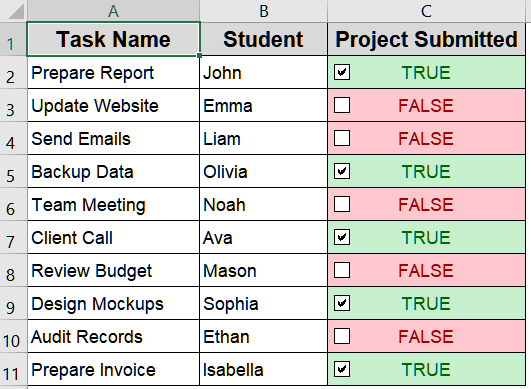
Applying Conditional Formatting Using Linked Cells
When a checkbox is inserted in Excel, it doesn’t hold a value by itself. To make it useful for conditional formatting, we link it to a cell. That cell then displays TRUE when checked and FALSE when unchecked. Conditional formatting rules can then target those TRUE/FALSE results to change formatting dynamically.
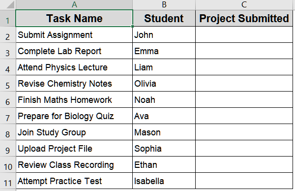
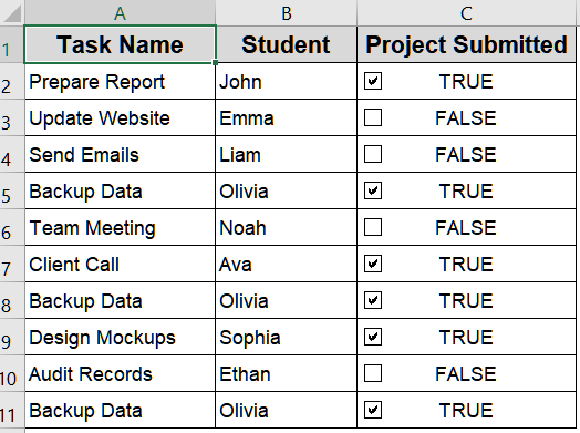
We’ll use the following dataset:
Steps:
➤ Insert a checkbox in column C using the Developer tab >> Insert option >> Form Controls >> Checkbox.
➤ Right-click the checkbox and select Format Control.
➤ In the Cell link box, select the cell where the checkbox state will be stored (e.g., C2) and click OK.
➤ Select the range of rows or cells you want to format (e.g., A2:C11).
➤ Go to Home >> Conditional Formatting >> New Rule.
➤ Choose Use a formula to determine which cells to format.
➤ Enter the formula:
=$C2=TRUE
➤ Click Format, select a fill color (e.g., green) to highlight completed tasks, then click OK twice.
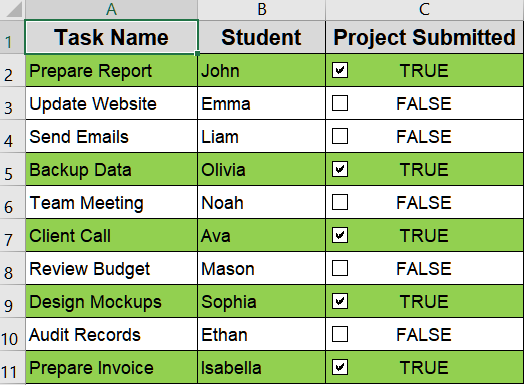
Now, whenever you tick a checkbox, the corresponding row will be highlighted.
Insert AND Formula to Highlight the Current Task
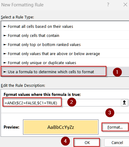
If your tasks are meant to be completed sequentially, you may want Excel to highlight the next task in line. Using an AND formula, you can identify the first unchecked item after a completed one which guides users to their next focus point. This is best suited for structured lists, instructions, or training steps that must follow a specific order.
Steps:
➤ Select A2:C11.
➤ Go to Conditional Formatting >> New Rule >> Use a formula to determine which cells to format.

➤ Enter the following formula:
=AND($C2=FALSE,$C1=TRUE)
➤ Click Format, and choose a light yellow fill or bold text.
➤ Click OK.
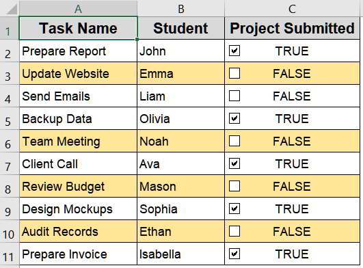
Now Excel will automatically highlight the next incomplete task right after a completed one.
Highlight Duplicate Tasks Using Conditional Formatting
You may occasionally need to check for duplicate entries (e.g., repeated task names or students). With a master checkbox, you can create a setup where duplicates are only highlighted when that checkbox is checked. This gives you control over when to display duplicate warnings without cluttering your sheet.
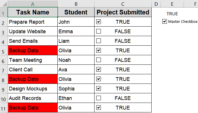
We’ll use the following modified dataset:
Steps:
➤ Insert a master checkbox from the Developer tab.
➤ Right-click the box to open Format Control and link it to a helper cell (e.g., E1).
➤ Select A2:A11 (Task Name column).
➤ Go to Conditional Formatting >> New Rule >> Use a formula to determine which cells to format.
➤ Enter this formula:
=AND($E$1=TRUE,COUNTIF($A$2:$A$11,A2)>1)
➤ Click Format >> Choose a red fill or border >> click OK.
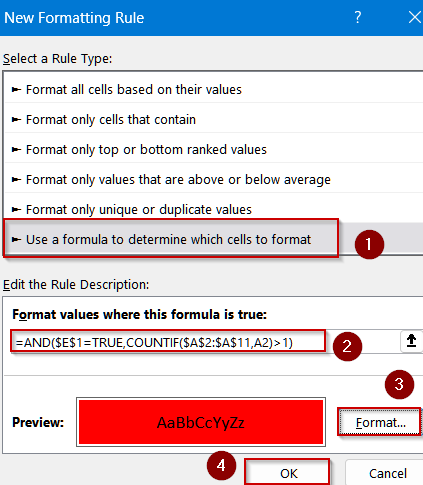
Now duplicates will highlight only when your master checkbox is checked.
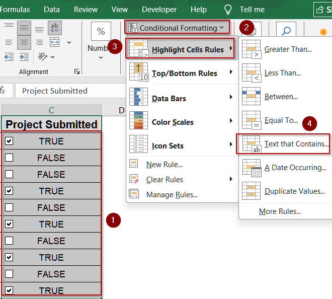
Conditional Formatting Using Text That Contains Feature
If you’re not working with checkboxes but instead use text markers like “TRUE” or “FALSE”, Excel’s built-in Text That Contains option is a fast and easy solution. You can apply colors or styles based on keywords. This is particularly useful for task lists imported from other systems or when you prefer plain-text updates instead of linked checkbox logic.
Steps:
➤ Select the range containing status text (e.g., C2:C11).
➤ Go to Home >> Conditional Formatting >> Highlight Cells Rules >> Text That Contains.
➤ Type TRUE or Done (depending on your data).
➤ Choose a format (e.g., green fill for TRUE).
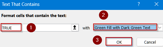
➤ Repeat for FALSE or Pending with a different color.
➤ Click OK to apply.
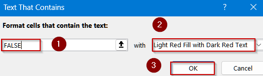
You’ll now have color-coded statuses that match your checkbox outcomes or textual inputs.
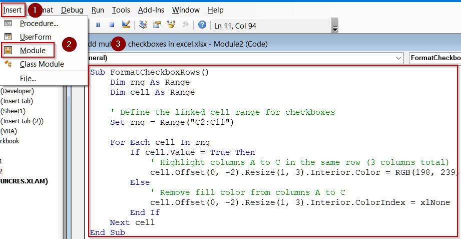
Automating Checkbox Formatting with VBA
When working with large datasets or frequently updated checklists, VBA (Visual Basic for Applications) can help you automate conditional formatting changes whenever a checkbox is toggled. This macro listens for changes in the linked cell values and automatically applies a specific format (like color) based on whether they are TRUE or FALSE.
Steps:
➤ Press Alt + F11 to open the VBA editor.
➤ Go to Insert >> Module.
➤ Paste the following code:
Sub FormatCheckboxRows()
    Dim rng As Range
    Dim cell As Range
    ' Define the linked cell range for checkboxes
    Set rng = Range("C2:C11")
    For Each cell In rng
        If cell.Value = True Then
            ' Highlight columns A to C in the same row (3 columns total)
            cell.Offset(0, -2).Resize(1, 3).Interior.Color = RGB(198, 239, 206) ' Light green
        Else
            ' Remove fill color from columns A to C
            cell.Offset(0, -2).Resize(1, 3).Interior.ColorIndex = xlNone
        End If
    Next cell
End Sub
➤ Close the VBA editor and return to Excel.
➤ Press F5 key to run the macro.
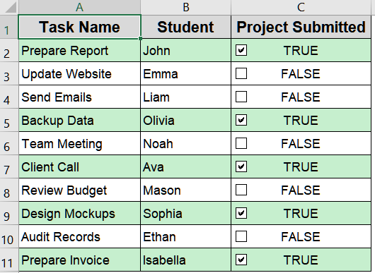
Each time you check or uncheck boxes, re-run the macro to update formatting automatically. You can also set it to run on worksheet change events for full automation.
Frequently Asked Questions
How do I make a checkbox control formatting automatically?
You can link each checkbox to a specific cell in Excel, then create a conditional formatting rule that references that linked cell, such as =C2=TRUE. This ensures formatting automatically updates when the checkbox is checked or unchecked.
Can I apply different colors for checked and unchecked boxes?
Yes, you can apply separate conditional formatting rules for different checkbox states. For example, use =TRUE for checked boxes (green) and =FALSE for unchecked boxes (red or no fill). This makes completed versus pending tasks visually distinct.
Do ActiveX checkboxes work with conditional formatting?
ActiveX checkboxes cannot directly trigger conditional formatting. Instead, link each checkbox to a cell that returns TRUE or FALSE. Then, base your conditional formatting rules on the values in those linked cells to control the formatting.
Can I automate checkbox formatting without re-running a macro?
Yes, you can use the Worksheet_Change event in VBA to automatically update formatting whenever a linked cell changes. This removes the need for manually running a macro, making your Excel sheet dynamically respond to checkbox changes.
Will conditional formatting rules work after saving and reopening the file?
Yes, conditional formatting rules persist even after saving and reopening your workbook. As long as the linked cells remain connected to their checkboxes, Excel will continue applying the formatting automatically whenever the checkbox states change.
Wrapping Up
In this tutorial, you learned how to apply conditional formatting to checkboxes in Excel using linked cells, relative referencing, using a master checkbox, Text that Contains feature and VBA automation. This feature can turn any static checklist into a dynamic tracker which is ideal for task management, attendance logs, or student progress sheets. Feel free to download the practice file and share your feedback.