Highlighting “Yes” and “No” in Excel with different colours helps make datasets more readable and visually appealing. It is especially helpful for displaying datasets with repetitive values, where quick identification is important. By using Excel’s built-in tools and options, we can easily perform this task.
Follow the steps below to highlight “Yes” as Green and “No” as Red in your dataset.
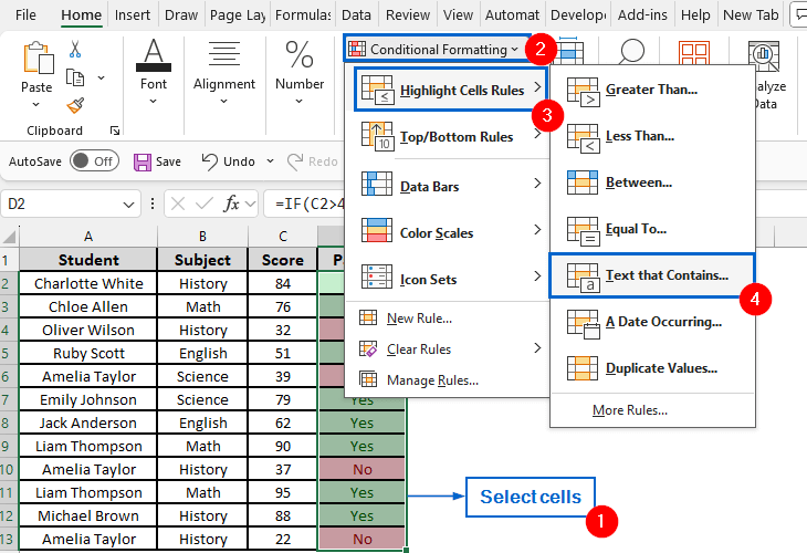
➤ Start by selecting the range of cells that you want to highlight, then from the main menu, head to Conditional Formatting >> Highlight Cell Rules >> Text that Contains.
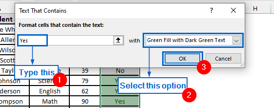
➤ Type “Yes” in the Format cells that contain the text field, then select Green Fill with Dark Green Text and click OK to highlight “Yes” in green.
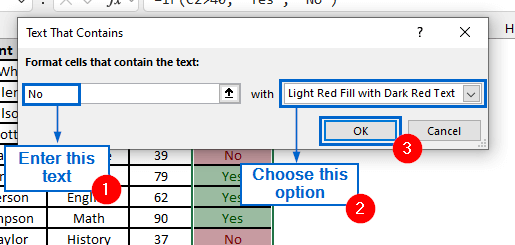
➤ Type “No” in the Format cells that contain the text field, then select Light Red Fill with Dark Red Text and click OK to highlight “No” in red.
In this article, we will learn five effective methods of making “Yes” green and “No” red in Excel.
Highlight Yes in Green and No in Red Using Conditional Formatting Highlight Cell Rules
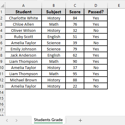
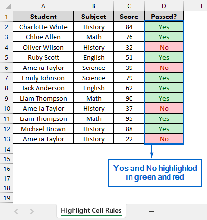
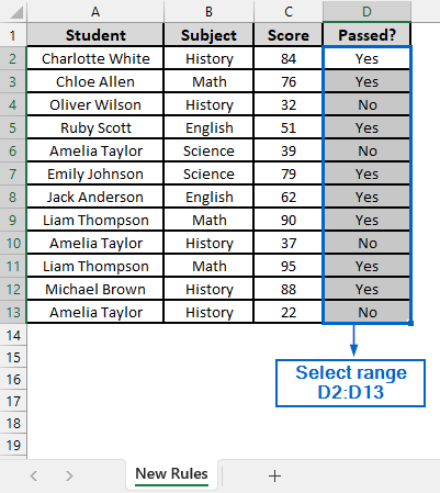
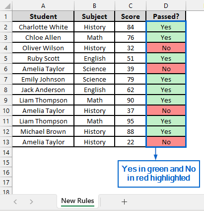
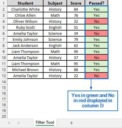
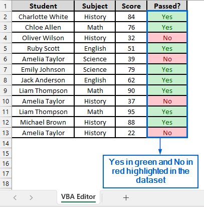
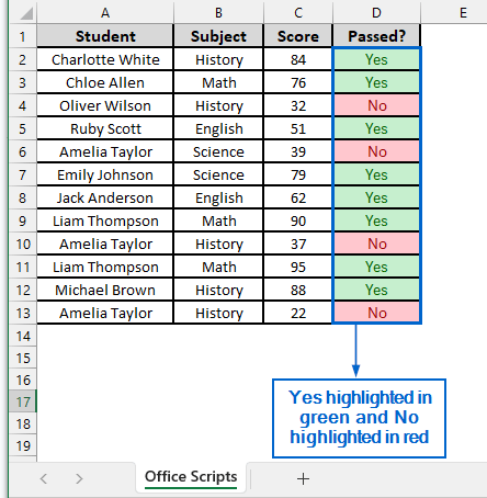
In the sample dataset, we have a worksheet called “Student Grades” containing information about Student names, Subject, Score, and their Pass status.
By using the Highlight Cell Rules option from the Conditional Formatting tool, we will format column D so that “Yes” appears in green and “No” appears in red in the dataset. We will display the updated dataset in a separate “Highlight Cell Rules” worksheet.
Highlight Cell Rules is a useful Excel feature that allows users to quickly format cells based on specific conditions, such as values greater than, less than, equal to, or containing certain text, dates, or duplicates.
Steps:
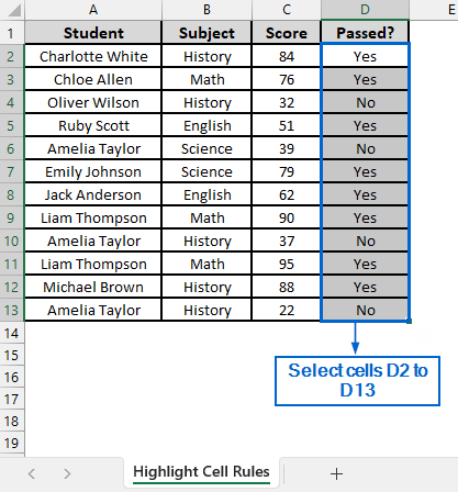
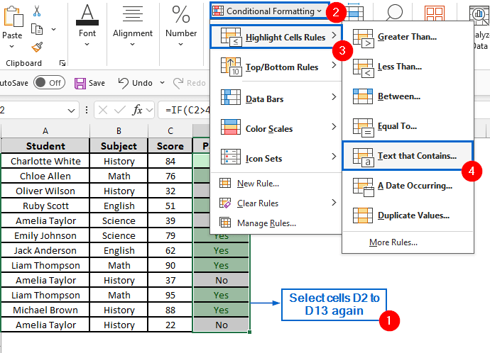
➤ Head to the Highlight Cell Rules worksheet and select cells D2 to D13.
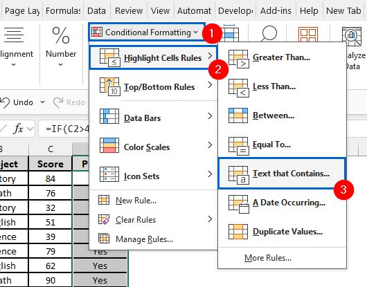
➤ Now, from the main menu, navigate to Conditional Formatting >> Highlight Cell Rules >> Text that Contains.
➤ Enter “Yes” in the Format cells that contain the text box, choose Green Fill with Dark Green Text, and click OK to format “Yes” in green.
➤ Again select cells D2 to D13 and head to Conditional Formatting >> Highlight Cell Rules >> Text that Contains from the main menu.
➤ Next, enter “No” in the Format cells that contain the text box, choose Light Red Fill with Dark Red Text, and click OK to format “No” in red.
➤ Your dataset should now highlight “Yes” in green and “No” in red.
Make Yes Green and No Red Using Custom Conditional Formatting Rules
Conditional Formatting is an important tool in Excel that allows users to automatically apply formatting such as colours, icons, or data bars based on user-defined cell rules.
Using the same dataset, we will now apply conditional formatting in column D by creating a new rule that highlights “Yes” in green and “No” in red. The updated dataset will be stored in a separate “New Rule” worksheet.
Steps:
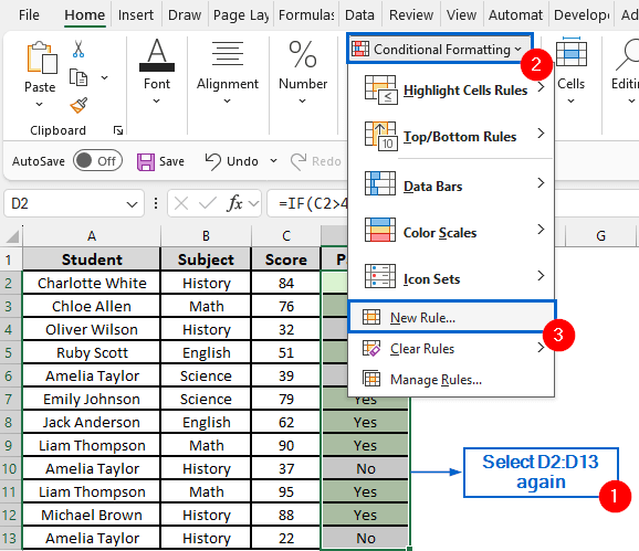
➤ Open the New Rule worksheet and select range D2:D13.
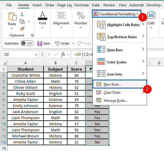
➤ From the main menu, head to Conditional Formatting >> New Rule.
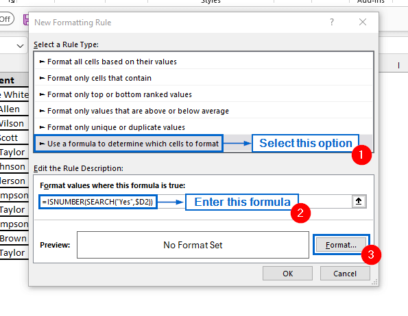
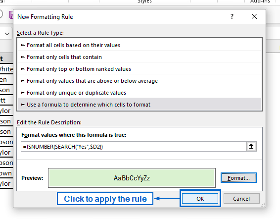
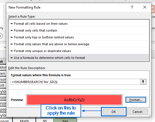
➤ From the New Formatting Rule dialogue box, select Use a formula to determine which cells to format option. Then, in the Format values where this formula is true field, enter the following formula and click Format:
=ISNUMBER(SEARCH("Yes",$D2))
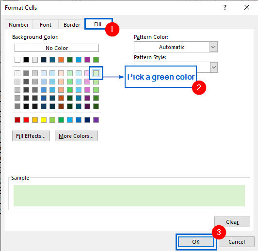
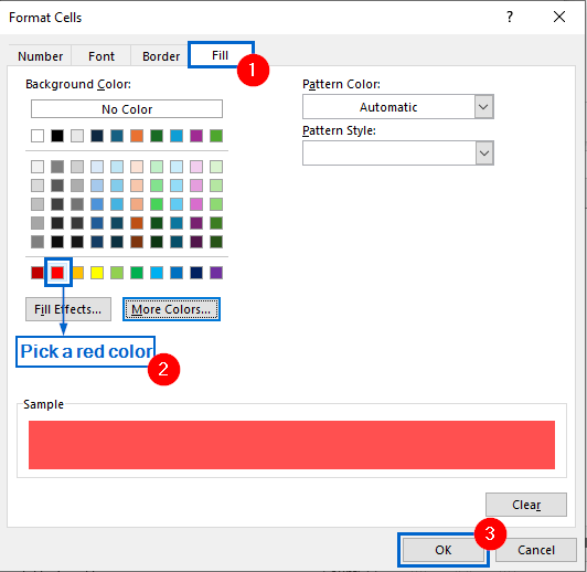
➤ Next, in the Format Cells dialogue box, go to the Fill tab, choose a green colour, and click OK.
➤ Finally, click OK in the New Formatting Rule dialogue box to apply the rule.
➤ Again select the range D2:D13 and head to Conditional Formatting >> New Rule.
➤ Select Use a formula to determine which cells to format option, enter the following formula under Format values where this formula is true field and click on Format.
=ISNUMBER(SEARCH("No",$D2))
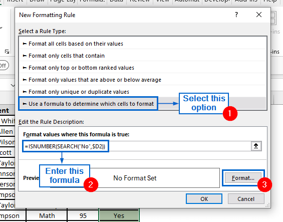
➤ Next, select red as fill colour from the Fill tab and click on OK.
➤ Click OK to complete the operation.
➤ The dataset should now highlight “Yes” in green and “No” in red.
Use the Filter Tool to Highlight Yes and No
The Filter Tool in Excel is a useful feature that allows users to display only the rows that meet specific criteria while temporarily hiding the rest.
Working again with the same dataset, we will now apply the Filter Tool to column D for highlighting “Yes” in green and “No” in red within the dataset. We will display the modified dataset in a separate “Filter Tool” worksheet.
Steps:
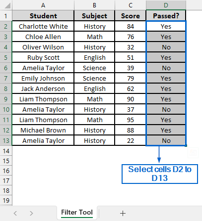
➤ Open the Filter Tool worksheet and select cells D2 to D13.
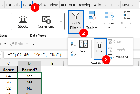
➤ Then, from the main menu, head to Data >> Sort & Filter >> Filter.
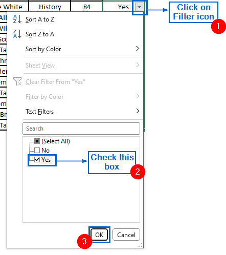
➤ Click the Filter icon next to cell D2, uncheck all options except “Yes” and click OK.
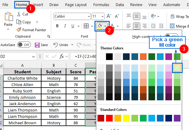
➤ Next, go to the Home tab, select a green fill colour, and apply it to all cells containing “Yes”.
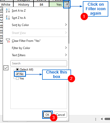
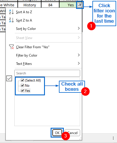
➤ Once again, click the Filter icon in cell D2, this time check only the “No” option, and then click OK.
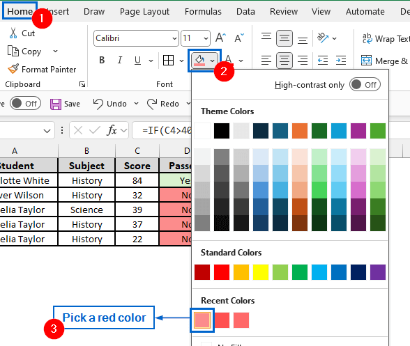
➤ Go to the Home tab again, select a red fill colour, and apply it to all cells containing “No”.
➤ Click Filter icon for the last time and check all boxes.
Note:
To remove the filter icon, select cells D2 to D13 and navigate to Data >> Sort & Filter >> Filter.
➤ “Yes” in red and “No” in green should now be visible in column D.
Automatically Highlight Yes Green and No Red Using VBA Editor
Excel’s VBA Editor is a powerful tool that allows users to write and run custom macros for automating tasks. We can also use it to automatically highlight cells with the colours we want, based on specific values or conditions.
Using the same dataset again, we will now use VBA Editor to highlight Yes and No values in column D in green and red, respectively. The modified dataset will be displayed in a separate “VBA Editor” worksheet.
Steps:
➤ Open the VBA Editor worksheet and press Alt + F11 to launch the VBA Editor window.
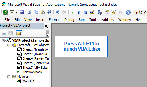
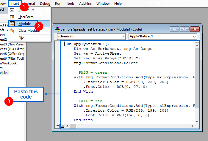
➤ In the Microsoft VBA Editor dialogue box, go to Insert >> Module from the main menu, and then paste the following code:
Sub ApplyStatusCF()
    Dim ws As Worksheet, rng As Range
    Set ws = ActiveSheet
    Set rng = ws.Range("D2:D13")
    rng.FormatConditions.Delete
    ' PASS = green
    With rng.FormatConditions.Add(Type:=xlExpression, Formula1:="=LOWER(TRIM($D2))=""Yes""")
        .Interior.colour = RGB(198, 239, 206)
        .Font.colour = RGB(0, 97, 0)
    End With
    ' FAIL = red
    With rng.FormatConditions.Add(Type:=xlExpression, Formula1:="=LOWER(TRIM($D2))=""No""")
        .Interior.colour = RGB(255, 199, 206)
        .Font.colour = RGB(156, 0, 6)
    End With
End Sub
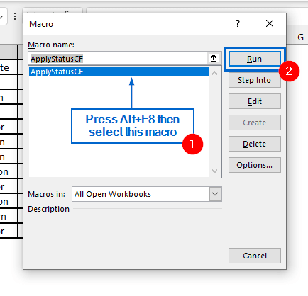
➤ Now, press Alt + F8 to open the Macros dialogue box, select the ApplyStatusCF macro, and click Run.
➤ “Yes” in green and “No” in red should now automatically be highlighted in the dataset.
Make Yes Green and No Red with Office Scripts
Office Scripts is another powerful tool in Excel that enables users to automate repetitive tasks, record actions, and create custom scripts for streamlining workflows.
We will use the same dataset and write an Office Script to automatically highlight the cells in column D with green and red colours. The updated dataset will be stored in a separate worksheet called “Office Script”.
Steps:
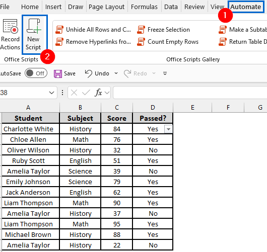
➤ Open the Office Script worksheet and from the main menu, head to Automate >> New Script.
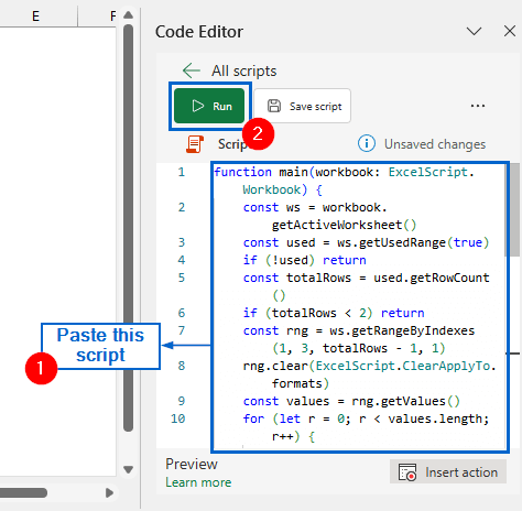
➤ In the Code Editor pane, paste the following script and click on Run:
function main(workbook: ExcelScript.Workbook) {
    const ws = workbook.getActiveWorksheet()
    const used = ws.getUsedRange(true)
    if (!used) return
    const totalRows = used.getRowCount()
    if (totalRows < 2) return
    const rng = ws.getRangeByIndexes(1, 3, totalRows - 1, 1)
    rng.clear(ExcelScript.ClearApplyTo.formats)
    const values = rng.getValues()
    for (let r = 0; r < values.length; r++) {
        const text = String(values[r][0]).trim().toLowerCase()
        const cell = rng.getCell(r, 0)
        const fmt = cell.getFormat()
        if (text === "yes") {
            fmt.getFill().setColor("#C6EFCE")
            fmt.getFont().setColor("#006100")
        } else if (text === "no") {
            fmt.getFill().setColor("#FFC7CE")
            fmt.getFont().setColor("#9C0006")
        }
    }
}
➤ The dataset will now automatically highlight “Yes” in green and “No” in red.
Frequently Asked Questions
What Happens If My Dataset Has Blank Cells in the Column?
For all the methods discussed in this article, blank cells in the column will be ignored by default. Conditional Formatting rules, and Filter only apply changes to cells that meet specific conditions, while VBA and Office Scripts skip over blank cells, applying formatting only to those containing actual values.
Which Method is Best For Large Datasets?
For large datasets, the VBA Editor and Office Script methods are the most efficient. They apply formatting automatically across the dataset, saving time and reducing manual effort.
Concluding Words
Knowing how to highlight “Yes” green and “No” red in an Excel dataset is crucial for improving data readability and analysis. In this article, we have discussed five effective methods on how to make yes green and no red in Excel, including using Conditional Formatting Rules, Filter Tool, VBA Editor and Office Scripts. Feel free to try out each method and select one that best aligns with your needs.