
In Excel, sometimes you need to find a specific piece of text or a character from a large string. For example, have you ever needed to find the 3rd dash in the Order ID? It might seem irrelevant at first, but it is also necessary while pulling out important information. To fix the messy dataset or analyze the product codes, extracting a specific character’s position can save you a lot of time. Sadly, Excel has no built-in function to find the nth occurrence of any character. But that does not mean you can’t find it.
To find the nth occurrence of character in string, follow the steps below: –
➤ Open the dataset, and find the cell (or cells) from which you need to extract the string.
➤ Identify the character that needs to be found.
➤ Use the FIND and SUBSTITUTE formula,
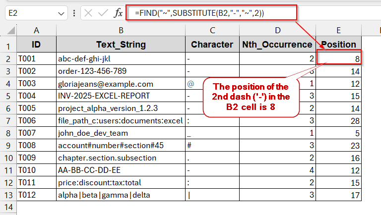
=FIND(“~”,SUBSTITUTE(B2,”-“,”~”,2))
Here, the 2nd dash (‘–’) is found in the B2 cell.
➤ Press Enter, and the FIND function to get the position of the 2nd dash.
➤ Do the same for the rest of the cells by dragging them. Or, replace the character in the SUBSTITUTE function as the first parameter.
And that’s not all. In this article, we’ll go beyond just one formula. We will discuss various formulas like FIND and SEARCH, as well as modern Excel 365 tools like TEXTSPLIT. You’ll also see how the helper columns can make this a lot easier and readable. Lastly, for advanced usage, we covered the Visual Basic (VBA) automated method to get this done as quickly as possible. Don’t rush, follow us as we dive deeper into each with interactive example datasets and a precise tutorial.
Get the Nth Occurrence Position of a Character Using SUBSTITUTE and FIND Functions
Though you can’t find the nth occurrence of any character with a single formula, you can combine the SUBSTITUTE and FIND functions to do that. The SUBSTITUTE function replaces the character that needs to be found from the mentioned position with a unique marker (often ‘~’). Wrapping the formula with the FIND, the unique marker’s position is found afterwards. This works in most of the Excel versions and is fast to implement.
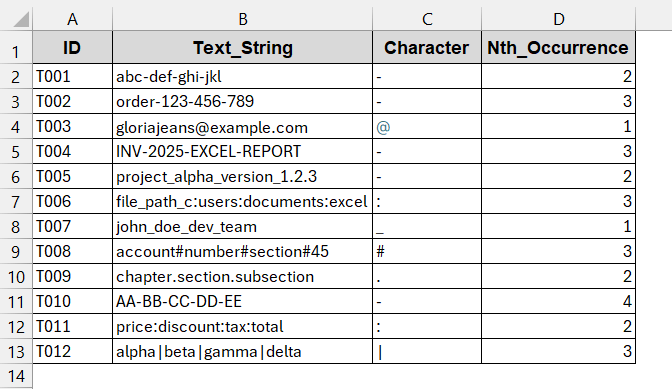
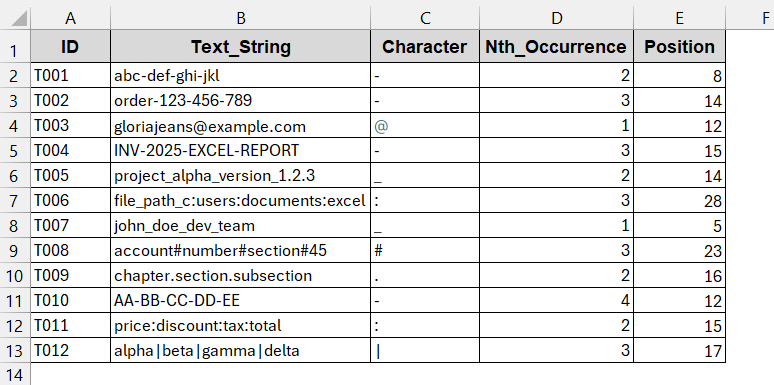
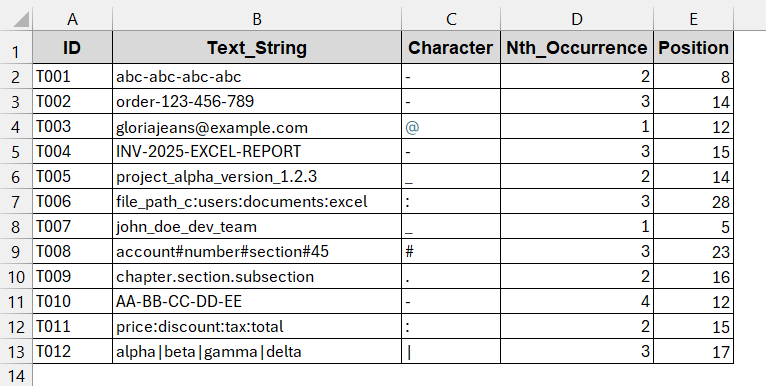
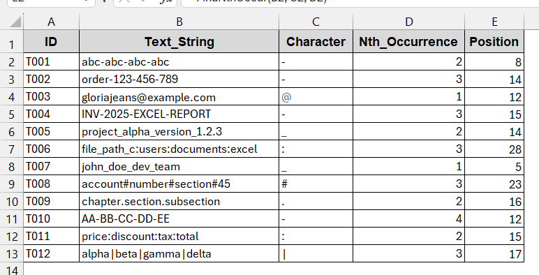
In this example, we have the following dataset. Here, from the Text_String, we will find the position of the Character mentioned in column C and the Nth_Occurrence from column D.
Steps:
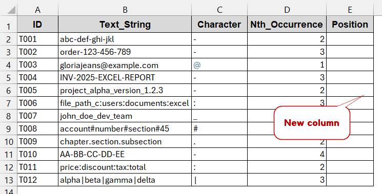
➤ Create a new column to store the position of the characters.
➤ In the first cell of the column, write the following formula –
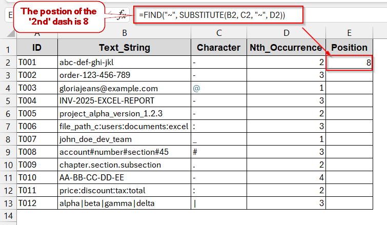
=FIND("~", SUBSTITUTE(B2, C2, "~", D2))
Here, the 2nd (D2) character in B2 (‘–’) is replaced with the unique marker (‘~’) by the SUBSTITUTE formula. The FIND function finds the position of the marker.
➤ Press Enter to get the value in the output cell.
➤ Drag the cells or use Fill Handle to generate the same formula for all the cells.
=IFERROR(FIND("~", SUBSTITUTE(B3, C3, "~", D3)), "Not found")
This will give Not found text in the output cell when the character is not present instead of #VALUE.
➨ The FIND function is case-insensitive, while the SUBSTITUTE function is case-sensitive.
➨ For data with mixed cases, use the LOWER formula to convert all the characters to lower cases by wrapping the cell references inside SUBSTITUTION.
=IFERROR(FIND(CHAR(1), SUBSTITUTE(LOWER(B4), LOWER(C4), CHAR(1), D4)), "Not found")
Using TEXTSPLIT and SEQUENCE Functions in Excel 365 for Finding Nth Occurrence
The FIND+SUBSTITUTE method is effective, but it gets complicated as you nest it with other formulas. This not only looks messy but also lags the performance of functions heavily for larger datasets. The good thing is that if you’re an Excel 365 user, you can get your hands on the TEXTSPLIT and SEQUENCE. Instead of a nesting formula, this formula splits the selected text string into nth parts based on the characters. Later on, it chose the part that is needed.
Steps:
➤ Open the datasets and identify the characters and the occurrences that need to be found.
➤ Create a new column to store the position of the characters (e.g., Position).
➤ In the first cell of the column, write the following formula –
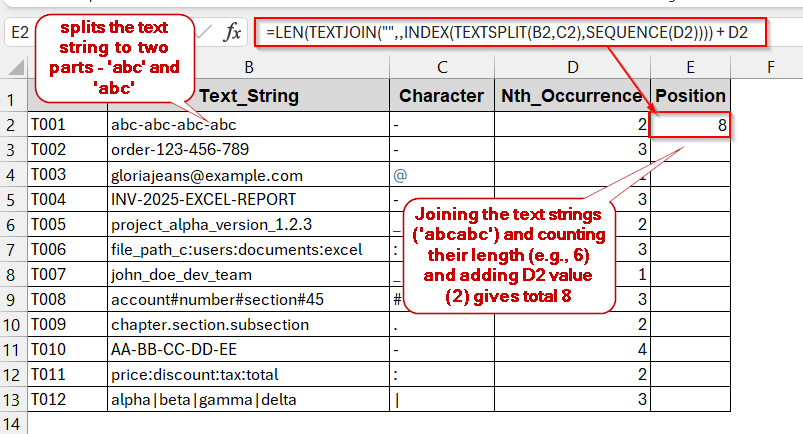
=LEN(TEXTJOIN("",,INDEX(TEXTSPLIT(B2,C2),SEQUENCE(D2)))) + D2
➨ The INDEX and SEQUENCE return the number of parts based on the nth occurrence. If the occurrence is 2, it will return only the first two parts, even if there are five split parts.
➨ The TEXTJOIN joins both the returned strings.
➨ LEN (..) + D2 finds the exact position of the occurrence of the delimiter.
➤ Press Enter to get the result.
➤ Drag the cells to apply the same formula to the rest of the column.
Notes:
➨ This method only works in Excel 365 and Excel 2021.
➨ Automatically spills the results into multiple columns due to its dynamic features.
Track Character Occurrence of Nth Position with FILTER & SEQUENCE Functions
Suppose the previous formulas do not work properly or look complex, worry not. There are still more formulas that you can try on. You can combine the classic SEQUENCE formula with the FILTER. This not only breaks the strings into parts based on the character, but it also filters and deletes duplicate values. Afterwards, wrapping them in INDEX can give you the exact position.
Steps:
➤ Open the dataset and determine the character and occurrence you need to find.
➤ Make another column to store the positions.
➤ Write the formula in the first cell of the column –
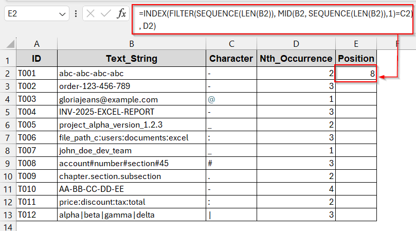
=INDEX(FILTER(SEQUENCE(LEN(B2)), MID(B2, SEQUENCE(LEN(B2)),1)=C2), D2)
where B2 is the text string, C2 is the character, and D2 is the nth occurrence of the character.
➤ Press Enter to get the result in the selected cell.
➤ Drag the cells to get the same formula implementation for the rest of the cells.
=FILTER(SEQUENCE(LEN(A2)), MID(A2, SEQUENCE(LEN(A2)),1)=B2)
➨ FILTER and MID only work in Excel 365. In other versions, use SMALL and IF.
=SMALL(IF(MID($B2,ROW($1:$100),1)=$C2,ROW($1:$100)),D2)
Create a VBA Function to Find the Nth Occurrence of a Character
As you can see, all the formulas are longer or shorter. It can really get messy when we add more items to this. The result is a huge performance issue, especially in the larger datasets. VBA is the most efficient and quick solution for solving this. You can actually create a custom function using the VBA Macros to pass three parameters of the selected string, character, and occurrence. The rest of the work is automatically done.
Steps:
➤ Open the dataset and create a column to store the position.
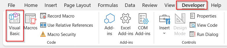
➤ Go to the Developers tab and click on Visual Basic.
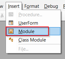
➤ It will launch the VBA editor window. In the window, click on the Insert tab -> Module
➤ Paste the below VBA code in the blank space-
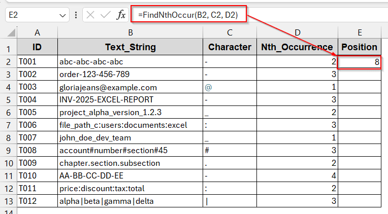
Function FindNthOccur(txt As String, ch As String, n As Long) As Variant
    Dim i As Long, count As Long
    FindNthOccur = CVErr(xlErrValue)
    For i = 1 To Len(txt)
        If Mid(txt, i, Len(ch)) = ch Then
            count = count + 1
            If count = n Then
                FindNthOccur = i
                Exit Function
            End If
        End If
    Next i
End Function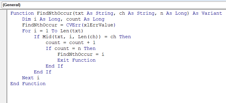
➤ Save the workbook as macro-enabled by Ctrl + S and click No to save.
➤ Close the window.
➤ Go back to the dataset.
➤ In the new column, use the VBA function –
=FindNthOccur(B2, C2, D2)
This function takes the string as the first parameter. The character that needs to be found in the second, and lastly, the nth occurrence as the third parameter.
➤ Press Enter.
➤ Use Fill Handle to apply the same formula to the rest of the cells.
Notes:
➨ This new function works for both single-character and multi-character strings.
➨ When the occurrence of the character does not exist, it gives #VALUE. You can modify the VBA script or wrap this formula with ISERROR to produce Not found when a character is absent in the nth occurrence.
Frequently Asked Questions (FAQs)
How do I extract the text after the nth occurrence of a character?
To find the nth occurrence and return everything after it, you can use the basic FIND and SUBSTITUTE functions combined with MID. Use the formula below-
=MID(B2, FIND(‘~’, SUBSTITUTE(B2, C2, ‘~’, D2)) + 1, LEN(B2)).
To find the text before the nth occurrence, use LEFT instead of MID.
Can I find the nth occurrence of multiple characters in the same string?
Excel does not have the option to find multiple character occurrences inherently. But, to work the way out, you can use the SUBSTITUTE formula as it replaces all of them with the same marker. As a result, the formula of FIND+SUBSTITUTE is enough.
How do I dynamically change the “n” in formulas without editing them each time?
To make the formula dynamic, use the cell references in the formula instead of the hardcoded text. If your formula looks like this –
=FIND((‘~’, SUBSTITUTE(‘abc-abc-abc-abc’, ‘-’ ‘~’, 2))
with this –
=FIND(CHAR(1), SUBSTITUTE(B2, C2, CHAR(1), D2))
Does this work with non-English characters or symbols?
All the above-mentioned methods worked with non-English characters and symbols as long as they are Unicode. However, be mindful of case-insensitive formulas and multi-byte characters.
Can Power Query be used to find nth occurrences?
For more advanced use cases, Power Query can also find the nth occurrence of the character. The column must be loaded in the Power Query editor window, and the column text needs to be split by Split Column by Delimiter. Text.Length will help you find the position afterward.
Concluding Words
Excel does not have a direct formula to find the nth occurrence of a character in string. Whether you prefer the classic approach of FIND and SUBSTITUTE functions or modern formulas like TEXTSPLIT, you get total control of parsing the texts in a different way. Also, to save yourself from all those hassles, you can create your own user-defined formula using VBA. As you explore all these methods, you’ll know that no method is the best. However, depending on the data size, your requirement, and character length, you can often find the perfect match for you.