Excel’s Macro Recorder and Visual Basic for Applications (VBA) can automate repetitive reporting tasks, turning hours of manual work into a simple click. Macros allow you to record complex sequences of actions and execute them instantly with a single click. By recording sequences of formatting and charting steps, you can instantly apply them to new datasets. In this article, we will provide a complete guide on how to automate reports using macros in Excel.
To automate reports using macros in Excel, here is one simple solution by recording macros and applying them.
➤ Record separate macros for distinct tasks like header formatting, conditional formatting, and creating chart.
➤ Use the Macros dialog box to quickly run all recorded macros on a new sheet of raw data to perfectly automate reports using macros.
Steps to Automate Reports Using Macros in Excel
Here, we will cover all the steps to automate reports using macros in Excel. We have broken down the process into the following steps: preparing the data, recording the three essential macros, and then executing them to create the automated report.
Step 1: Creating Raw Dataset
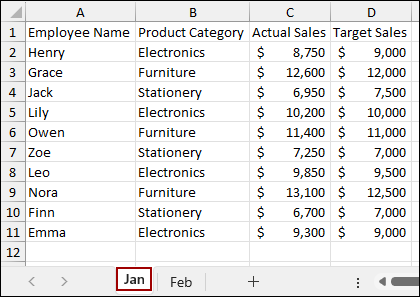
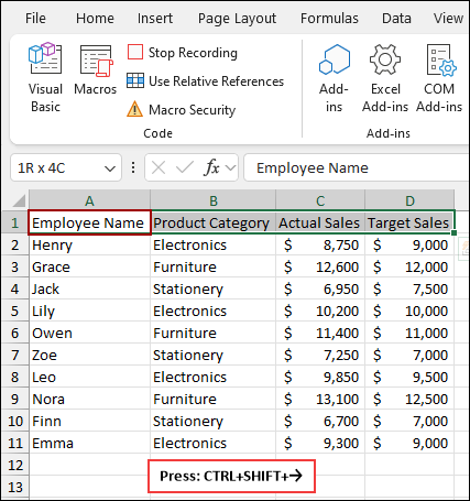
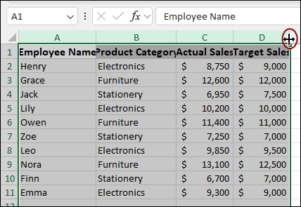
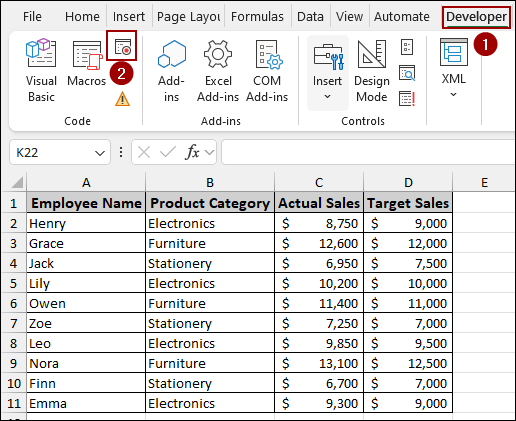
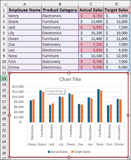
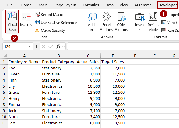
First, we will create the dataset. Suppose we have the following data in a sheet named Jan: Employee Name, Product Category, Actual Sales, and Target Sales for January.
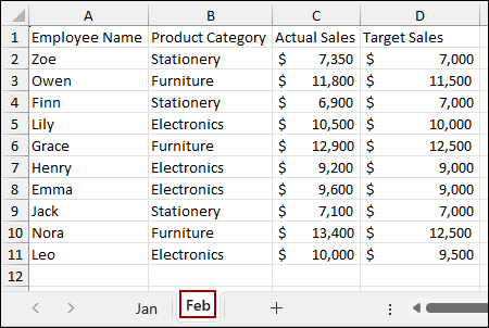
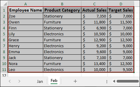
In another sheet named Feb, we have the same column but different data for February.
Step 2: Recording the Header Formatting Macro
In the Jan sheet, we will start recording a macro to automate the common formatting steps for the report header.
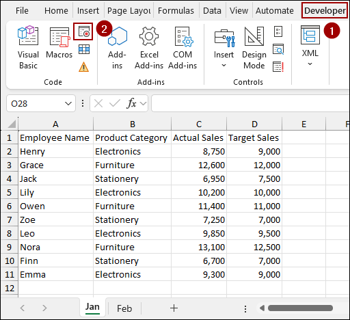
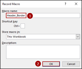
➤ Navigate to the Developer tab and click on the Record Macro icon.
➤ In the Record Macro dialog box, give your macro a clear name, such as Header_Border, and click OK.
Remember that macro names cannot contain spaces.
Every action we perform will be recorded in the macro.
Let’s start with the header formatting.
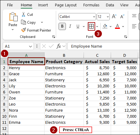
➤ Select the header row, which is A1:D1, by clicking on cell A1 and pressing Ctrl + Shift + → .
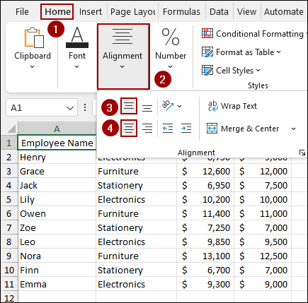
➤ Go to the Home tab to change the text alignment.
➤ Under the Alignment group, click the Center Alignment option and then the Middle Align option to center the text within the header cells.
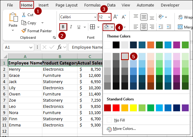
➤ Go to the Home tab, make the header text Bold, and change the Font Size to 12.
➤ Next, click the Fill Color dropdown and select a light grey color to highlight the header row.
➤ To adjust the column widths to fit the content, select all the columns (A:D) and double-click on the crosshair icon.
➤ Now, select the entire dataset by clicking on any cell within the data (like A1) and pressing Ctrl + A .
➤ Click the Borders dropdown under the Font group and select All Borders to apply borders to the data.
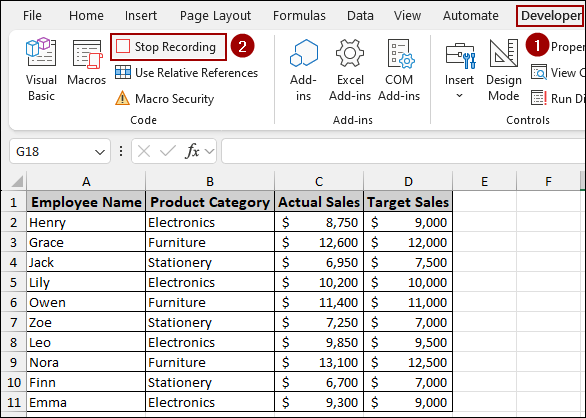
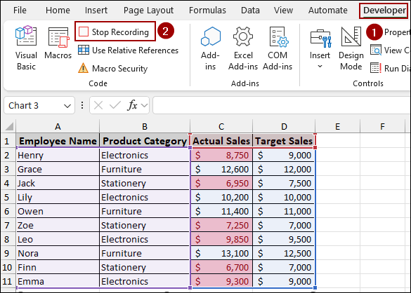
Once all the formatting steps are complete, we must stop the recording.
➤ Go back to the Developer tab.
➤ Click on Stop Recording in the Code group.
Before moving on, it’s a good practice to check whether the macro recorded properly or not.
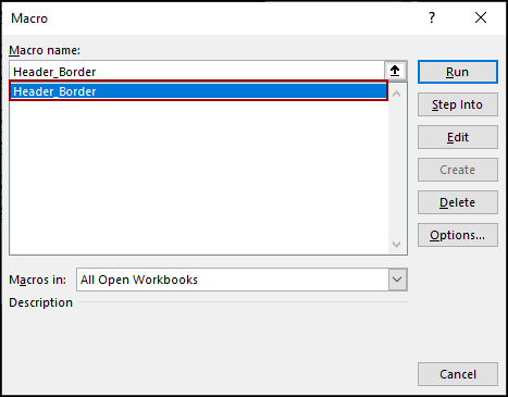
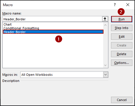
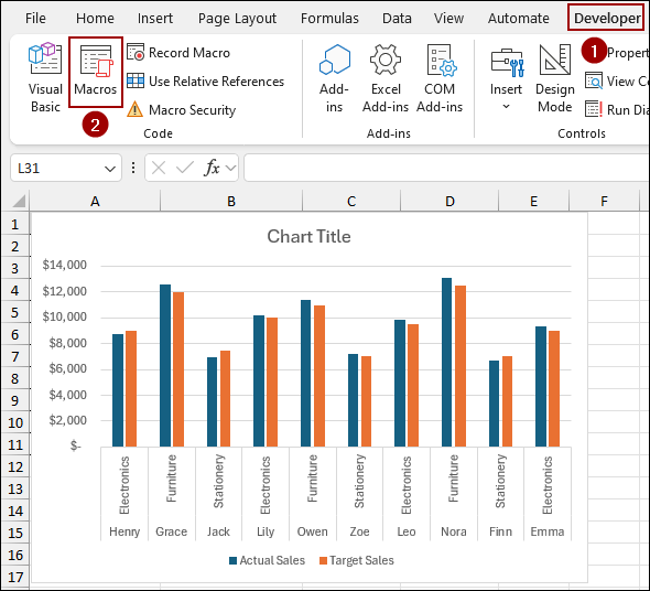
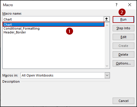
➤ Go to the Developer tab and click Macros to open the Macro dialog box.
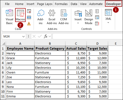
In the Macro dialog box, we will see the macro with the name Header_Border is recorded.
Step 3: Recording the Conditional Formatting Macro
In this step, we will record the second macro to automatically apply conditional formatting.
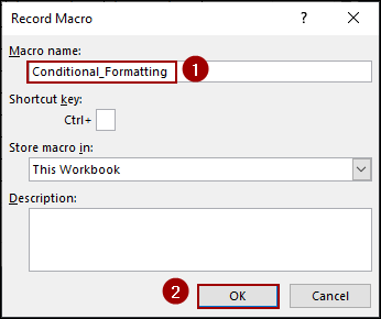
➤ Click the Record Macro icon on the Developer tab.
➤ Name this new macro Conditional_Formatting and click OK to begin recording.
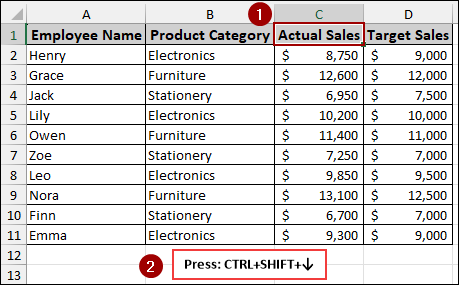
➤ Select the range of sales data in column C (starting from C2) by clicking on cell C2 and pressing Ctrl + Shift + ↓ .
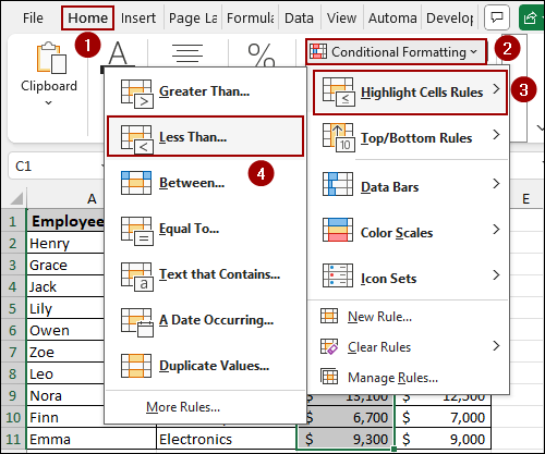
➤ Go to the Home tab, click the Conditional Formatting dropdown, hover over Highlight Cells Rules, and select Less Than.
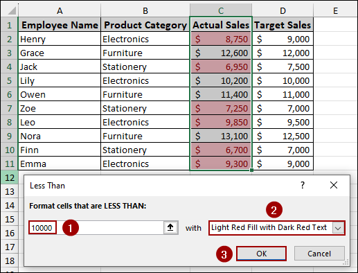
➤ In the Less Than dialog box, enter the value, such as 10000, in the text field.
➤ Ensure the formatting is set to Light Red Fill with Dark Red Text and click OK.
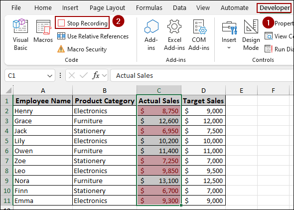
Once the conditional formatting is applied, stop the recording to save the steps.
➤ Go back to the Developer tab.
➤ Click on Stop Recording.
Step 4: Recording the Chart Generation Macro
To complete the report automation, we will create a third macro to instantly generate a sales chart from the data.
➤ Go to the Developer tab and click Record Macro.
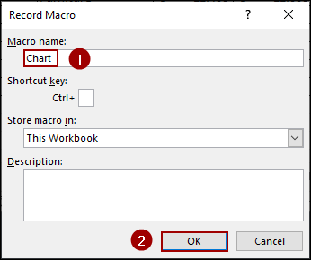
➤ Name this new macro Chart and click OK to begin recording the charting steps.
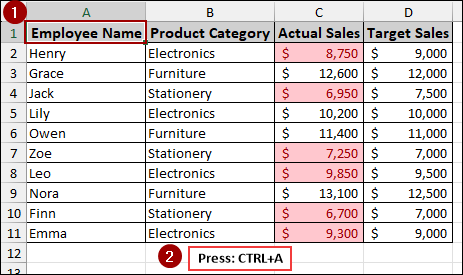
➤ Select the entire data range, including the header, by clicking on cell A1 and pressing Ctrl + A .
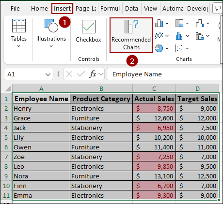
➤ Go to the Insert tab.
➤ Click on Recommended Charts.
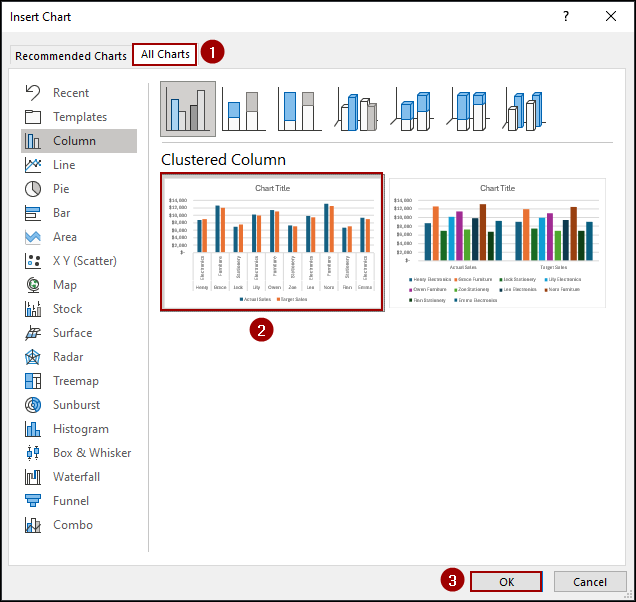
➤ In the Insert Chart dialog box, navigate to the All Charts tab.
➤ Select the Column type and choose the standard Clustered Column chart.
➤ Click OK to insert the chart onto the sheet.
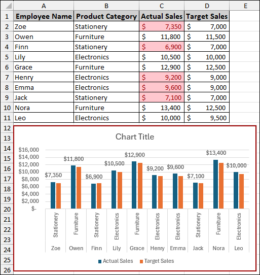
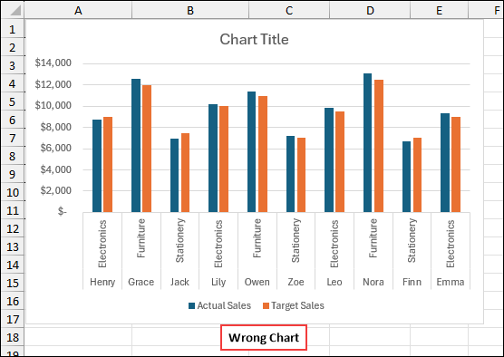
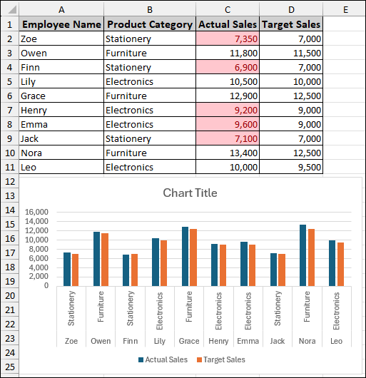
The new chart will appear, visualizing the Actual Sales versus Target Sales for all employees.
Now that the chart is created and formatted, you can stop the recording.
➤ Go back to the Developer tab.
➤ Click Stop Recording.
Step 5: Running Macros to Create Report in a New Sheet
We now have three powerful macros to automate our report generation. Let’s test them on the raw data for the next month, February.
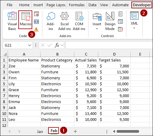
➤ Click on the Feb worksheet tab to activate the new raw data.
The February data is unformatted.
➤ Go to the Developer tab and click Macros.
➤ First, select the Header_Border macro from the list and click Run.
The macro will run and format the header, and apply borders to the data.
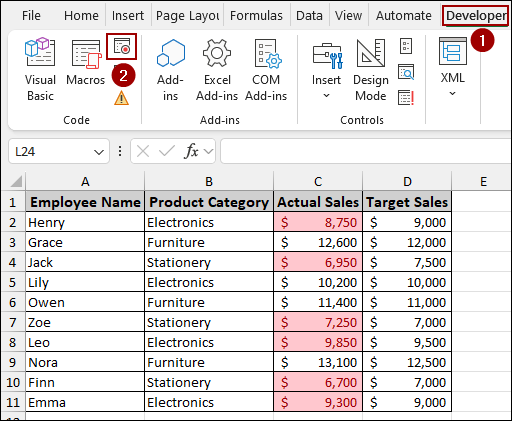
➤ Next, select the Conditional_Formatting macro from the list and click Run.
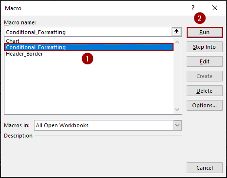
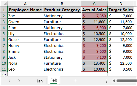
The macro will instantly apply the formatting and color highlighting to the February data.
When you try to run the third macro on the new data, you may encounter an issue where the chart is either blank or shows incorrect data because the recorded macro used static cell references.
➤ With the February data selected, run the Chart macro.
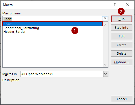
As a result, you will get an error or the chart showing the data from the Jan sheet.
Step 6: Fixing a Common Chart Macro Error
To fix this, we need to modify the VBA code to use a range that automatically adapts to the number of rows in the new dataset.
➤ Go to the Developer tab and click Macros.
➤ Select the Chart macro and click the Edit button.
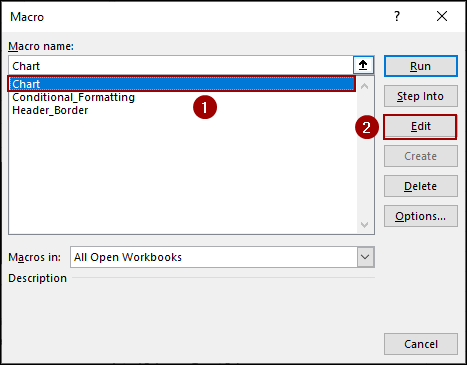
The Microsoft Visual Basic for Applications window will open, showing the recorded code for the chart macro.
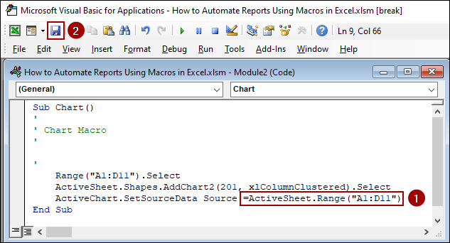
➤ For the ActiveChart.SetSourceData Source line, change the next part with the below code.
=ActiveSheet.Range(“A1:D11”)
➤ Click the Save icon in the VBA editor to save the changes.
After fixing the issue, let’s run the chart macro again.
➤ Go to Developer > Macros, select the Chart macro and click Run.
The final result is a complete, well-formatted, conditionally highlighted report with a correct chart.

Instead of running each macro individually, you can use a simple VBA code to execute all three with a single click.
➤ Go to the Developer tab and click Visual Basic (or press ALT + F11).
➤ Insert a new module, paste the code and Run it.
Sub Run_All_Report_Macros()
Call Header_Border
Call Conditional_Formatting
Call Chart
End Sub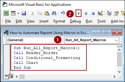
As a result, with just a single click the code will format the header, apply conditional formatting, and create the chart, fully automating the report.
Frequently Asked Questions
Can I automate reports from multiple sheets or files?
Absolutely. VBA can loop through multiple sheets or workbooks, consolidate the data, and generate a combined report automatically.
Why is my macro not running in another computer?
Macros may be blocked due to security settings. Go to File > Options > Trust Center > Trust Center Settings > Macro Settings, and enable macros to allow them to run.
Can I trigger macros with a button or shortcut key?
Yes. You can insert a Form Control Button from the Developer tab or assign a keyboard shortcut while recording your macro for quick access.
Concluding Words
Above, we have covered all the steps to automate report in Excel. By recording the macro in small parts and applying those you can reduce the time spent on report generation. Remember that the key to macro use is consistency in your raw data structure and checking the code for fixed ranges. If you encountered any issues, especially with the chart, revisit the VBA editing steps to ensure your code is dynamic. If you have any questions, please don’t hesitate to share them in the comments section below.