
When managing data in Excel, you may sometimes want to make one drop-down list depend on another. For example, when you select a Category like Fruit, you want the next drop-down to show only related Items such as Apple, Banana, or Orange. This type of setup is called a dependent or conditional drop-down list, and it helps keep data entry accurate and efficient.
In this article, you’ll learn how to create an Excel filter drop-down list based on a cell value using both traditional and modern methods.
Here’s how to create an Excel filter drop-down list based on a cell value:
➤ Open your dataset in Excel.
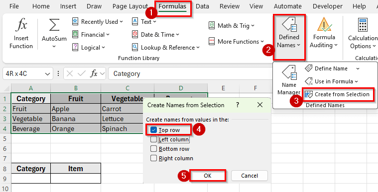
➤ Select A1:D4 and go to Formulas >> Define Names >> Create from Selection. Check Top row and click OK.
➤ In cell A9, create the first drop-down using Data >> Data Tools >> Data Validation >> List, and set the source to =Category.
➤ In cell B9, create the dependent drop-down using Data Validation >> List, and set the source to =INDIRECT(A9).
➤ Now, when you select a category in A9, B9 will show only the related items.
Create a Dynamic Drop-Down List Based on a Cell Value Using FILTER and UNIQUE
In the following dataset, we have product category information. Column A lists the Category, Column B shows the Item Names, and Column C contains their Prices. Columns F and G are empty, where we’ll create two drop-down lists. One for selecting a category and another that automatically filters items based on the chosen category.
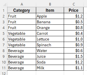
We’ll use this dataset to demonstrate different ways to create an Excel filter drop-down list based on a cell value.
If you are using Excel 365 or Excel 2021, you can create a dynamic filter drop-down list using the FILTER and UNIQUE functions. This modern method automatically updates the drop-down lists when you add new categories or items, so you do not have to redefine named ranges manually.
Here’s how to do it:
Step 1: Extract Unique Categories
➤ Open your dataset in Excel.
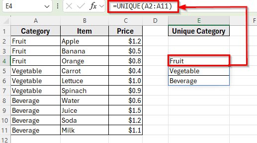
➤ Click on an empty cell, for example E4, and enter the following formula:
=UNIQUE(A2:A11)
➤ Press Enter. Excel will display a list of unique categories such as Fruit, Vegetable, and Beverage. This will serve as the source for the first drop-down list.
Step 2: Create the Primary Drop-down List
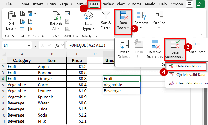
➤ Click on cell E2, go to the Data tab, and click Data Tools >> Data Validation.
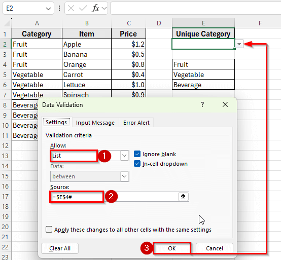
➤ Set Allow to List. In the Source box, type:
=$E$4#
➤ Click OK.
➤ The # symbol tells Excel to include all the values generated by the UNIQUE function.
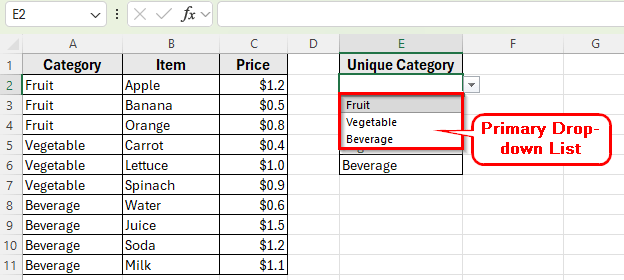
➤ Now cell E2 contains a dynamic list of categories.
Step 3: Filter Items Based on the Selected Category
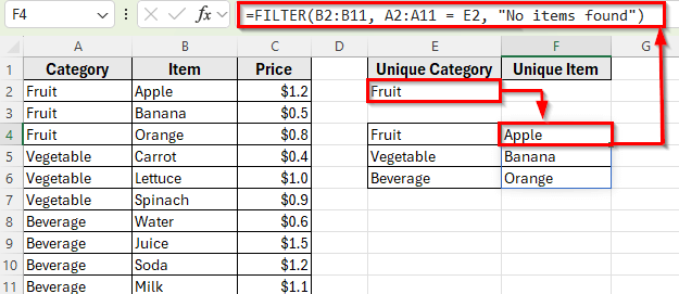
➤ Click on cell F4 and enter this formula:
=FILTER(B2:B11, A2:A11 = E2, "No items found")
➤ Press Enter. Excel will return only the items that match the category selected in E2. For example, if E2 is Fruit, you’ll see Apple, Banana, and Orange appear in cells starting from F4.
Step 4: Create the Dependent Drop-down List
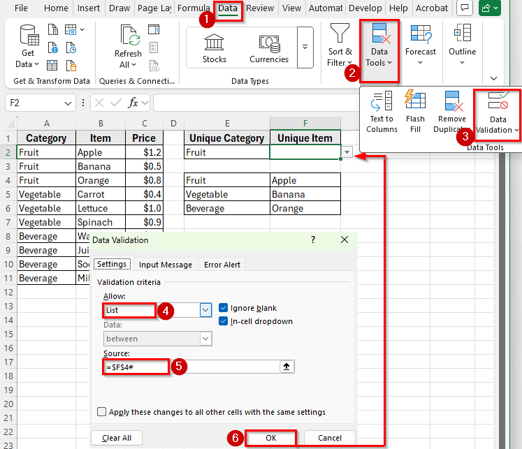
➤ Click on cell F2, go to the Data tab and click Data Tools >> Data Validation, and select List.
➤ In the Source box, type:
=$F$4#
➤ Click OK.
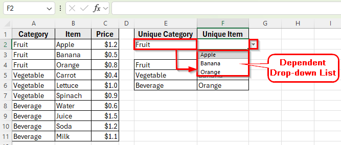
➤ Now, when you pick a category in E2, the second drop-down in F2 will only display items related to that category.
Step 5: Sort or Clean the Results.
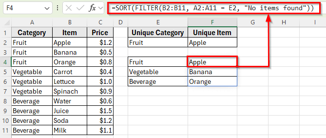
➤ If you want the list to appear alphabetically, modify the FILTER formula as follows:
=SORT(FILTER(B2:B11, A2:A11 = E2, "No items found"))
➤ This will sort the items in ascending order inside the spill range.
Step 6: Test the Setup
➤ Now test your dependent drop-down list.
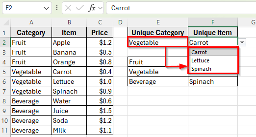
➤ Select Vegetable in cell E2. The second drop-down in F2 will show Carrot, Lettuce, and Spinach.
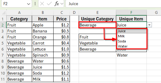
➤ Change E2 to Beverage. The F2 drop-down will instantly update to show Water, Juice, Soda, and Milk.
➤ This confirms that your formula and validation are working correctly.
Using Named Ranges and the INDIRECT Function
The most common way to create a filter drop-down list based on another cell’s value is by using named ranges and the INDIRECT function. This method is simple and works in all Excel versions. It allows the second drop-down list to display only the items related to the category selected in the first drop-down.
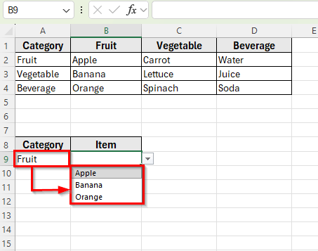
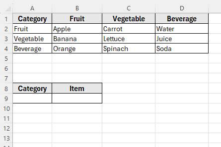
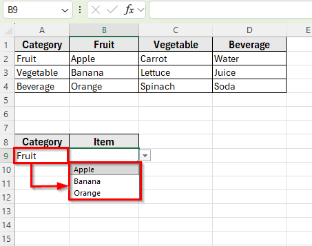
In this following dataset, we have a list of food categories and their corresponding items. Column A shows the Category, Columns B to D list specific items for each category such as Fruit, Vegetable, and Beverage. Below the table, cells A8 and B8 are labeled Category and Item, where we’ll create a dependent drop-down list.
Here’s how to do it:
➤ Open your dataset in Excel.
➤ Select your data range such as A1:D4 to define the name range for each list.
➤ Go to the Formulas tab and click Define Names >> Create From Selection.
➤ A window will appear, check the option Top row then click Ok.
➤ Make sure that each name exactly matches the category name used in your dataset, as this link is what makes the drop-down work correctly.
➤ Click on cell A9 where you want the first drop-down Category to appear.
➤ Go to the Data tab, click Data Tools >> Data Validation.
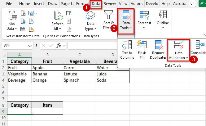
➤ Choose List as the validation type. In the Source box, type = and then press F3 from your keyboard. Select the name Category. Click Ok.
➤ Again click OK.
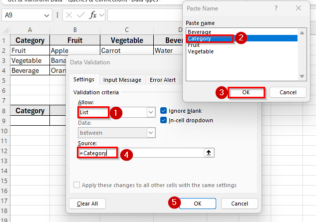
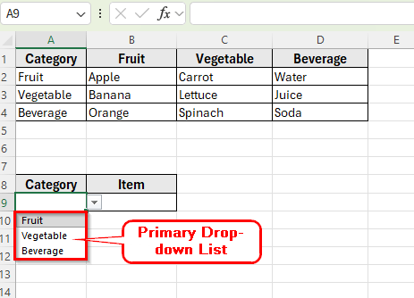
➤ Now, cell A9 will display a primary drop-down list of available categories.
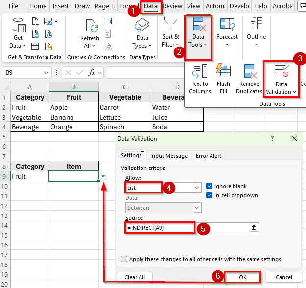
➤ Next create the dependent drop-down list. Click on cell B9 where you want the second drop-down (Item) to appear.
➤ Open Data Validation again and choose List as the validation type.
➤ In the Source box, enter the formula:
=INDIRECT(A9)
➤ Press OK. This formula tells Excel to use the named range that matches the selected category in A9.
➤ Next, test the drop-downs. Click the arrow in cell A9 and select Fruit. When you click the arrow in B9, it should now show Apple, Banana, and Orange.
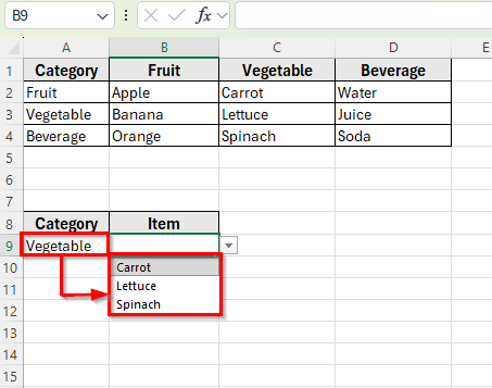
➤ If you change cell A9 to Vegetable, cell B9 will automatically display Carrot, Lettuce, and Spinach.
Downloadable Resources
Get our practice workbook or necessary files that we have worked with to prepare this article.
Filter Drop Down List Based on Cell Value.xlsx
Frequently Asked Questions
Can I use this method in older versions of Excel?
No. The FILTER and UNIQUE functions are only available in Excel 365 and Excel 2021. For older versions, you can use the Named Ranges and the INDIRECT function.
How do I make the drop-down list automatically expand when new items are added?
If you are using dynamic array formulas like UNIQUE and FILTER, Excel will automatically expand the spill range when you add new rows. You do not need to manually update the data validation source.
Why is my dependent drop-down list not updating automatically?
If your dependent drop-down list does not change after selecting a different category, you may have used a static range instead of a dynamic one. Make sure your formulas use the # symbol, for example, =$E$4#, in the Data Validation source box so Excel includes the entire dynamic spill range.
Wrapping Up
Creating a filter drop-down list based on a cell value in Excel helps you organize and analyze data more efficiently. In this guide, we used two practical methods such as one with Named Ranges and INDIRECT, and another using modern FILTER and UNIQUE functions.
The first method offers a fully dynamic solution that updates automatically as your data grows. And the second method is ideal for older Excel versions as all versions of Excel don’t accept FILTER function. By applying these techniques, you can make your Excel sheets more interactive and easier to navigate.