Google Sheets is a useful tool for task tracking, data organization, and collaboration with teammates. Google Sheets is very simple and makes data management accessible for both individual and group members in a team. When multiple members are working on the same sheet, or when the information is significant, then you need to protect the data. Google Sheets has easy-to-use tools to protect the data and ensure security. In this article, we will learn about how to protect Google Sheets in many ways.
Lock Entire Google Sheets with a Password
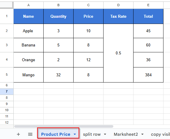
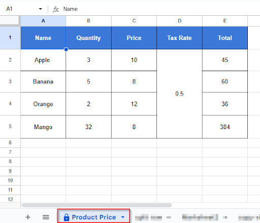
When you need to share a Google Sheet with somebody, but you don’t want them to change any of the data. Then you have to lock Google Sheets from editing. Google Sheets does not have a built-in password lock feature, but you can keep your information safe by restricting access, which acts as a virtual password. While still working together, you can lock individual cells, ranges, or even the entire sheet in Google Sheets. Look at the dataset below, where you want to lock the entire sheet and can simulate password-style security.
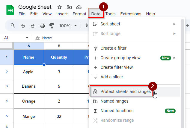
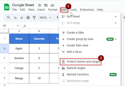
➤ Go to Data > Protect sheets and ranges.
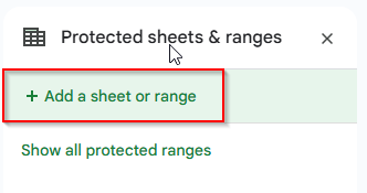
➤ Click Add a sheet or range.
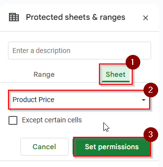
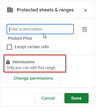
➤ Click on the Sheet tab and choose the entire sheet name “ Product Price”, then click Set permissions
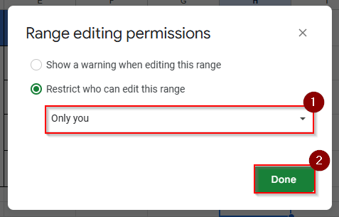
➤ Choose Only you can edit and click Done.
➤ Now the entire sheet is locked, and the editor can’t edit unless you give access. This works as a password.
Set Google Sheets Permissions Per Sheet
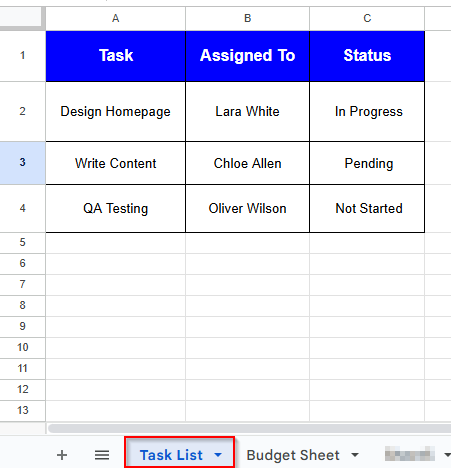
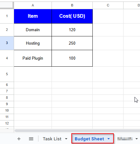
Although Google Sheets is an effective tool for teamwork, sometimes you don’t want to change your data or sheets by anyone. If you have multiple sheets to manage, you can set permissions for every sheet who can edit which sheet. At the same time, you can collaborate with your teammates, and you can also protect sensitive information in your Google Sheets. Let’s look at the two datasets below, where you want your team to edit the Task List sheet but not touch the Budget sheet.
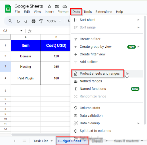
Here’s the Budget sheet:

➤ Click on the “Budget Sheet” you want to protect
➤ Go to Data > Protect sheets and ranges.
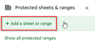
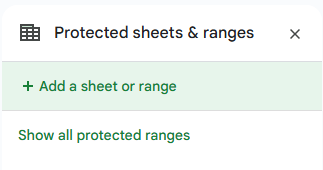
➤ In the sidebar, click “+ Add a sheet or range.”
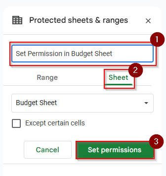
➤ Add a description like “Set Permission in Budget Sheet” and select the Sheet, then choose Budget Sheet. Click “Set Permissions” to set your permissions.
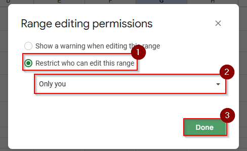
➤ Select Restrict who can edit this range > Only You, and click Done.
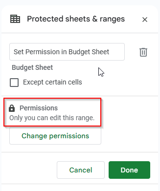
➤ Now, only you can edit the Budget Sheet.
Protect a Worksheet from View and Hide from Others
When you want to share a single Google Sheets worksheet but want to keep some of the important sheets hidden, such as internal notes or sensitive financial information. You can hide sheets from others and set permissions on who can see. You can’t fully limit sheet viewing on a per-user basis in Google Sheets. Let’s look at the two datasets below, where you want to share only the Task List sheet but keep the “Budget Sheet” hidden.

First of all, you have to set permissions. Don’t give edit access to anyone. To set permissions, you have to do:
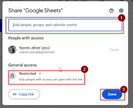
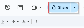
➤ Click Share.
➤ Set team members as Viewers or Commenters
➤ Under General access, select Restricted and click Done.
➤ Right-click on the “Budget Sheet 2” tab.
➤ Click “Hide sheet“.
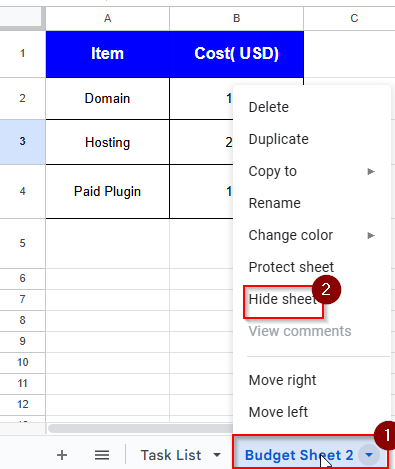
The Sheet is hidden from anyone who doesn’t have edit access.
Edit Permissions in Google Sheets
When you are working on a shared Google Sheet, you may want to give permissions to some members to view only certain parts, others to edit everything, and still others to edit everything. Editing permission in Google Sheets is very simple. It’s an ideal way for teamwork and data protection, and also your spreadsheet will remain clean, secure, and collaborative. Let’s look at the dataset below, where you will edit permissions.
➤ Click Share.
➤ Under “People with access”, you’ll see a list of who can view/edit the sheet.
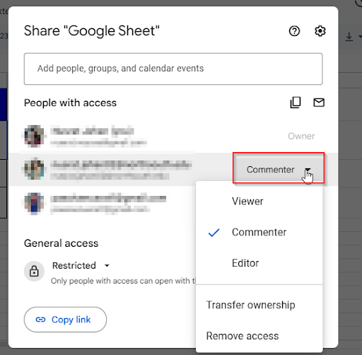
➤ Click the drop-down next to their name.
➤ Choose Viewer – Can only view the file, Commenter – Can view and leave comments, Editor – Can view and make changes.
➤ Then Click Done.
Protect Columns in Google Sheets
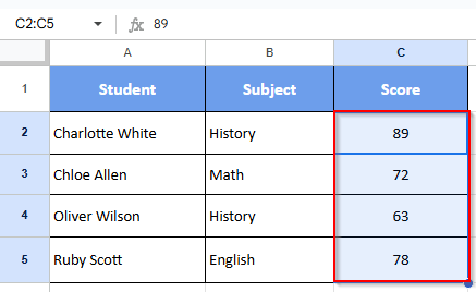
Important or sensitive information can be stored in specific columns in a shared Google Sheets. You don’t want the column should not altered by everyone. You can make certain columns inaccessible to anybody while the remainder of the sheet remains editable to anyone. Let’s look at the dataset below, where you want to protect the “Score” column, so others can’t change it accidentally.
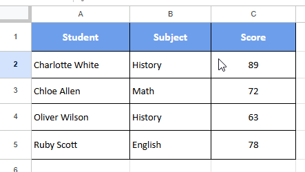
➤ Select cells C2:C5
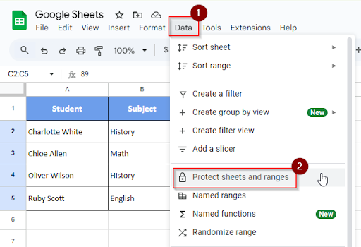
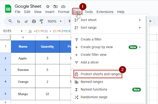
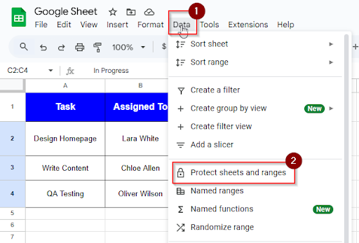
➤ Click on Data > Protect sheets and ranges.
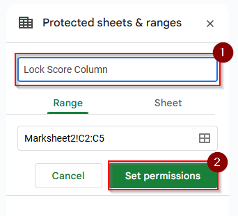
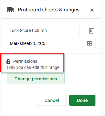
➤ Add a description in your protected range like “Lock Score Column“, and click “ Set Permissions”.
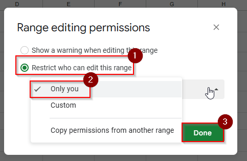
➤ A pop-up message will appear. Click on “ Restrict who can edit this range”. Choose an option to set permission: Only you , or Custom to allow specific users and click Done.
➤ Now the range is protected and locked. You can see that only you can edit this range. It works as a password.
Protect Formulas in Google Sheets
When you are sharing your spreadsheet, collaborators can edit your sheet. But you don’t want to change your formulas by anyone. So, you want to protect your formulas from others. You can easily protect formulas in Google Sheets so that other people can enter data without restriction while the logic remains unaltered. Let’s look at the dataset below, where column E is written with formulas.
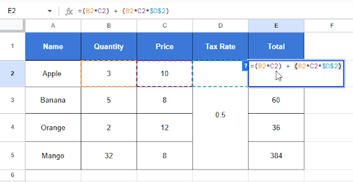
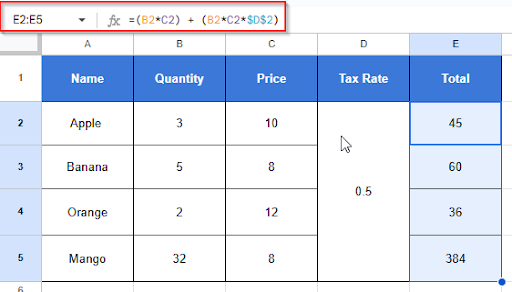
➤ Select all formula cells E2:E5
➤ Go to Data > Protect sheets and ranges.
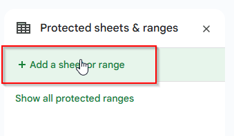
➤ In the sidebar, click “Add a sheet or range”.
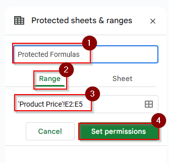
➤ Enter a name like Protected Formulas.
➤ Select Range Option.
➤ Confirm the selected range E2:E5
➤ Click “Set permissions”.
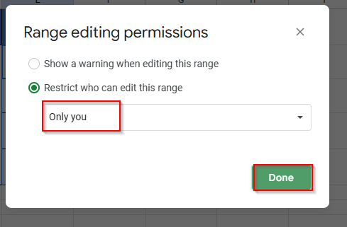
➤ Choose the “Only you” option to allow yourself to edit formulas and click Done.
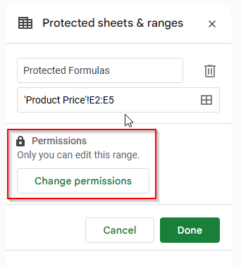
➤ Now you can see the result in the sidebar. Only you can edit the formula column. Formulas are protected from other users.
Fix the Protect Range Option Not Showing in Google Sheets
When you want to prevent editing of important data, such as pricing or calculations, you have to protect a range in Google Sheets. Sometimes “Protect sheets and ranges” option is available from the Data menu. You can solve this problem in many easy ways.
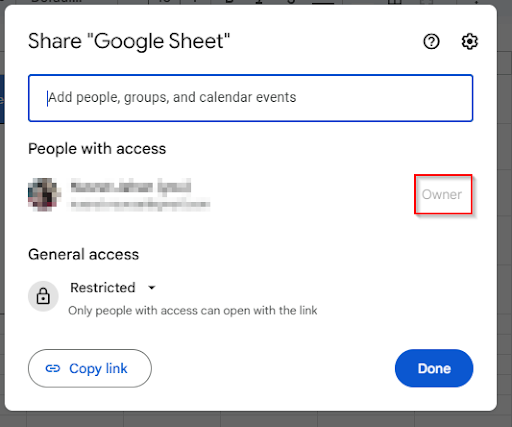
➤ Click on the Share option
➤ Check If You’re the Owner or Editor. You need to be the owner of this sheet or have editing access to show the protect range option.
Unprotect a Sheet in Google Sheets
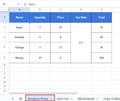
When you’ve applied protection to a sheet or certain cells in Google Sheets, and now you want to unprotect that sheet or certain cells. You have to follow simple steps to unprotect a sheet in Google Sheets. Let’s look at the dataset below, where you have protected the product price sheet.
➤ Click on the menu: Data > Protect sheets and ranges.
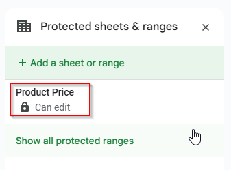
➤ You’ll see a list of protected ranges or sheets on the right side of the screen.
Click on the protected sheet name or range you want to unprotect.
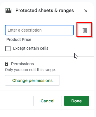
➤ Click the trash bin icon.
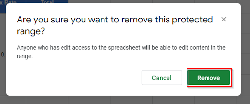
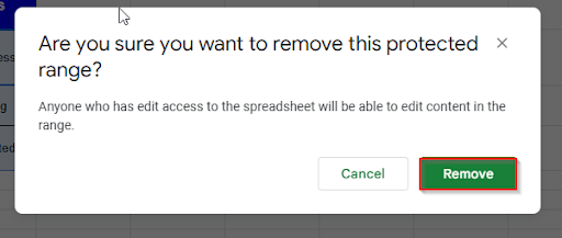
➤ Confirm by clicking Remove.
➤ Now you will see that the sheet is unprotected.
Unprotect Cells in Google Sheets
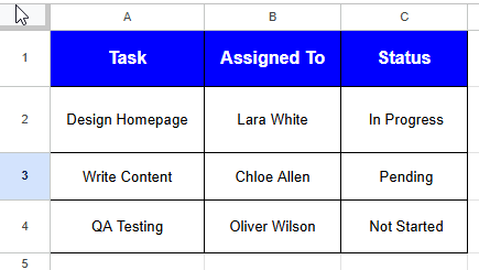
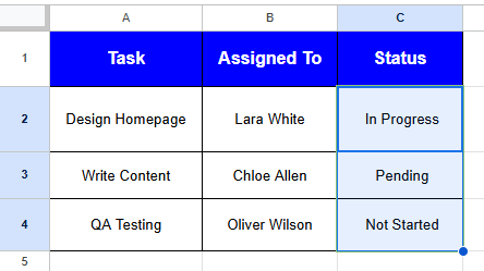
If you’ve protected some cells, and now you want to remove the protection from those cells. You can quickly remove or change the protection in Google Sheets to stop undesired edits and allow editing again. Let’s look at the dataset below, where the C2:C4 cells are protected.
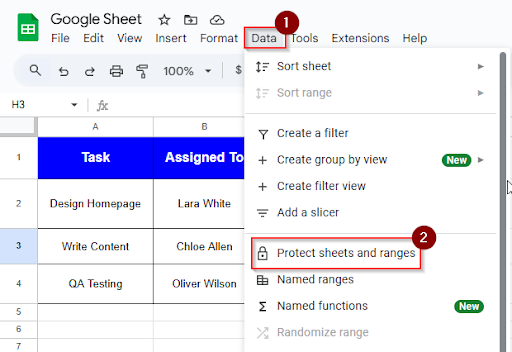
➤ Click Data > Protect sheets and ranges from the top menu.
➤ A sidebar will appear on the right, showing all protected ranges and sheets. Look for the name or range “ Task List! C2:C4”
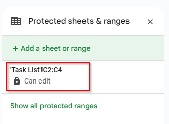
➤ Click on it once to select.
➤ Click the trash bin icon at the top of the box.
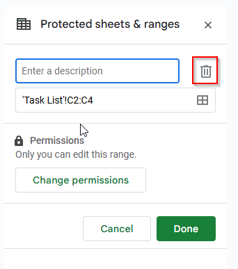
➤ Click Remove to confirm.
Now you can see that the protected cell range lists are removed.
Remove All Protected Ranges in Google Sheets
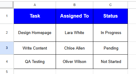
If you have protected multiple ranges, such as locked cells, columns, and now you want to remove all protected ranges in Google Sheets, you can do it easily by following the simple steps. But there is no ” Remove all ” button in Google Sheets. You have to do it one by one. It only takes a few minutes to remove multiple ranges. Let’s look at the dataset below, where you have the protected “Assigned to” and “Status” columns.
➤ Click on Data > Protect sheets and ranges.
➤ A sidebar will open on the right, and you’ll see a list of all protected ranges and sheets.
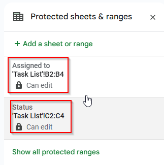
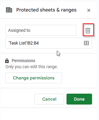
➤ Click on “Assigned to”
➤ Then click the trash bin icon.
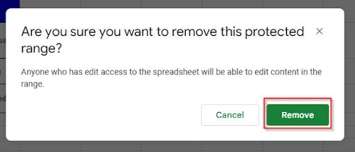
➤ Confirm by clicking Remove.
➤ Repeat this for “Status” cell ranges.
Frequently Asked Questions
Can viewers see the locked cell range?
Of Course. Viewers can view but can’t edit the locked cell range.
Can I hide an entire Google Sheet from specific users?
Not entirely. Although you can limit editing and hide a sheet.
Concluding Words
When you are working together in a Google Sheets, you need to protect your Google Sheets to avoid unintentional changes from other users. You can work together more confidently when you’re locking entire sheets, individual cells, or formulas. You can set permissions for individual users to protect your Google Sheet if you are the file owner.