Calculating running averages for time-based data is best for long-term projects, sales analysis, and recognizing changing trends. Here, we take a certain period and calculate the average of our data.
After combining several averages, we can easily see the changing patterns and avoid minor fluctuations. You also get to use an Excel chart to visualize the data points. While there are many ways to get running averages, using the Data Analysis ToolPak is the best way to automate the process.
➤ A running average is a statistical calculation that analyzes trends by averaging a subset of data points over a specified period.
➤ To calculate the running average, go to the Data tab >> Data Analysis. From the dialog box, Moving Average >> Ok.
➤ As the Moving Average window opens, select the Input Range for moving averages, the Interval to specify the period, and the Output Range for putting the calculated averages.
➤ If you want a graphic visual display, check the Chart Output box and click Ok.

In this article, we’ll cover what a moving average is and how to use it using different methods like the Analysis ToolPak and functions like AVERAGE, OFFSET, SUM, and COUNT.
What Is Running Average in Excel?
A running (or moving/rolling) average in Excel is an average calculation that updates as new data is added. It shows the average of a specific number of data points (e.g., last 3 months’ sales) or the average from the beginning up to the current point (cumulative).
Running averages are commonly used in sales trends, stock market analysis, quality control, and forecasting to smooth out fluctuations and reveal patterns.
Apply the AVERAGE Function to Determine the Cumulative (Overall) Running Average
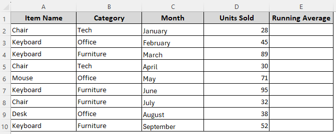
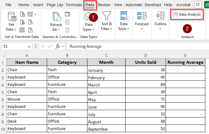
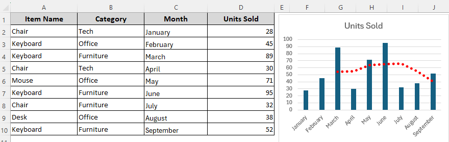
Our sample dataset includes rows for product names, category, months, and units sold per month. The data we want to use for our calculation is in the cells D2:D10. We’ll use Column E to calculate the running averages.
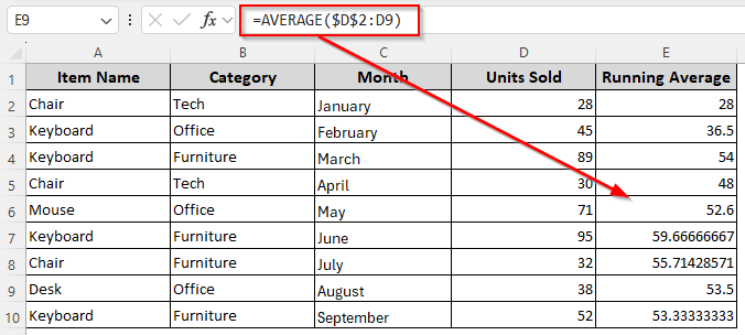
The cumulative running average refers to the average of all values from the first data point up to the current row. It shows the overall trend over time as more data is added. To see how the average changes over time as new data is added, we’ll use the AVERAGE function in the following way:
➤ In cell E2 (first row of average), enter the following formula:
=AVERAGE($D$2:D2)
➤ $D$2 is the fixed start point for the calculation and D2 changes as we drag down.
➤ Replace the references with the first cell of your data. Make sure you use an absolute reference (like $D$2) for the first cell reference.
➤ Press Enter and drag the formula down using the fill handle (+ sign on the bottom corner of the cell) to automatically calculate the running averages of all values from the first to the last row.
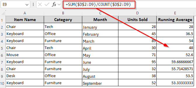
Determine Cumulative Running Average with the SUM and COUNT Functions
Another way to get a cumulative running average is to use the SUM and COUNT functions. If you want a running average from the start of the data up to the current row, follow these steps:
➤ In a cell of the running average column, type the following formula:
=SUM($D$2:D2)/COUNT($D$2:D2)
➤ As D2 is the first cell of our data range, we used $D$2:D2 in our formula. Change it as needed.
➤ Click Enter and drag the formula down.
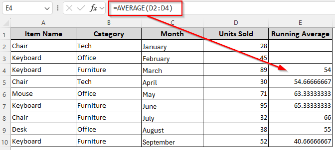
Calculating Simple Moving Average (SMA) with the AVERAGE Function
SMA refers to the average of a fixed number of recent periods (rolling window). It smooths short-term fluctuations and shows the underlying trend. We’ll calculate the moving average every 3 months. You can use the same method for a fixed period of days, months, or years. Below are the details:
➤ Choose the 3rd cell of the column (last cell of the range D2:D4) for running average, insert any of the following formulas:
=AVERAGE(D2:D4)
➤ Cell D2:D4 contains data for the first 3 months. Add or reduce cell numbers depending on the fixed number of previous periods you want to average.
➤ For example, we’ll change our range to D2:D6 for a 6-month running average. Also, you need to insert the formula in cell D6 (last cell of our range D2:D6) as we don’t have enough data in the first 5 cells to calculate the 6-month average.
➤ Click Enter and drag the formula down to apply it to subsequent cells.
Using the AVERAGE Function with COUNT and OFFSET for Dynamic SMA Average
If you keep adding new data and don’t want to update the range manually, you can combine the AVERAGE, COUNT, and OFFSET functions. While the OFFSET function dynamically shifts the range down as you drag the formula, the COUNT function counts how many numbers are from the start of the list up to the current row.
Let’s use them to calculate row-by-row rolling average for every N number of entries and only the most recent ones:
➤ Type any of the following formulas in the first row of the rolling average column:
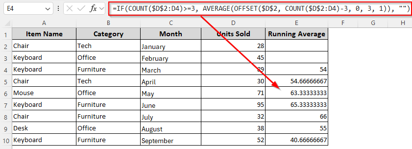
For Row-by-Row Running Average of N Values
To calculate the average of every 3 months from the start to the end, use this formula:
=IF(COUNT($D$2:D2)>=3, AVERAGE(OFFSET($D$2, COUNT($D$2:D2)-3, 0, 3, 1)), "")
➤ Here, D2 is the first cell containing the data we’re averaging and 3 is the number of months we’re averaging. Change them according to your dataset.
➤ Press Enter and drag the formula down to get the running averages every 3 months starting from the first cell. As we used the IF and COUNT functions to avoid errors and replace them with blanks, the first two cells are empty for lack of data to average.
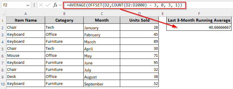
For the Latest N Values of a Column Only
➤ To get only the averages for the last 3 entries of your dataset, use this formula:
=AVERAGE(OFFSET(D2,COUNT(D2:D2000) - 3, 0, 3, 1))
➤ D2 is the first cell containing our data and D2:D2000 is the limit up to which this formula will adjust the result automatically. As we used 3, it will calculate the average of the last 3 cells only. Change these values as required.
➤ Press Enter and Excel will return the average for the latest 3 entries of your dataset. When you add new data, the average will be updated automatically up to cell E2000.
Automate Calculations and Display Graphics with the Data Analysis ToolPak
To calculate the average of a fixed number of periods, we can use the Data Analysis ToolPak in the following way:
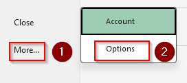
➤ To enable ToolPak, go to the File tab >> More >> Options.
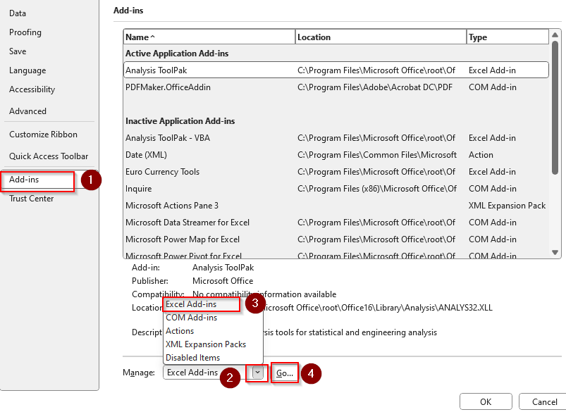
➤ Click on Add-ins from the side column. From the Manage drop-down choose Excel Add-ins and press Go.
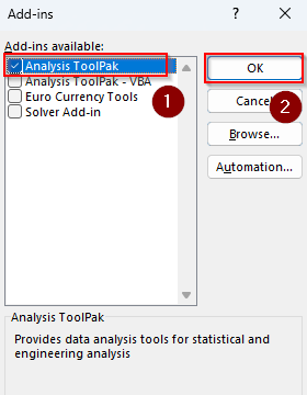
➤ In the Add-ins window, check Analysis ToolPak and click Ok.
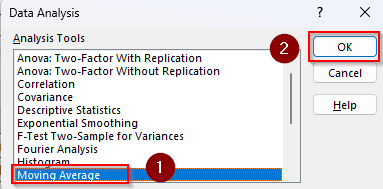
➤ Now, open the Data tab >> Data Analysis.
➤ When the Data Analysis dialog box appears, click on Moving Average >> Ok.
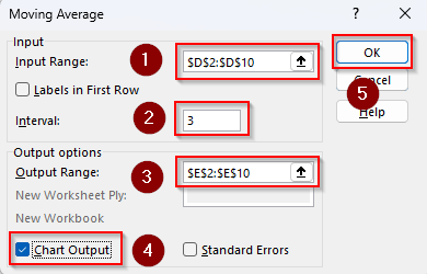
➤ From the Moving Average window, click the arrow beside the empty Input Range field and highlight the range containing the data you’re averaging. We’re selecting D2:D10.
➤ In the Interval box, manually type the number of periods to set data points. For example, we entered 3 for a 3-month average.
➤ Choose a new range in a blank column where the results should appear. We’re highlighting the E2:E10 range.
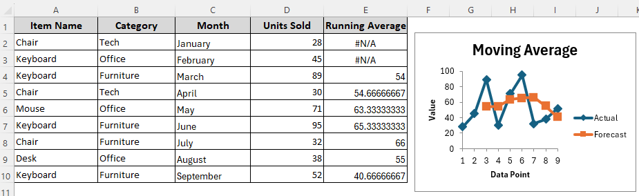
➤ Check the Chart Output box to add a graphic chart visualizing the moving average info. Finally, click Ok.
➤ Here’s the final result:
Determine Weighted Moving Average (WMA)
In WMA, we multiply N number of values with different weights so that recent data has a greater influence on the average. It’s useful when newer data matters more than older data.
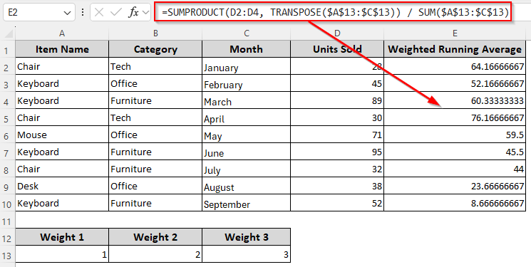
For this method, we entered 3 weights (1, 2, 3) in cells A13, B13, and C13. We’ll take 3 values starting from the top and multiply the oldest ones by the value in A13, the second oldest one by B13, the newest one by C13.
After that, using the SUMPRODUCT and SUM functions will calculate the running averages. Here are the details:
➤ Insert the following formula in a running average column cell:
=SUMPRODUCT(D2:D4, TRANSPOSE($A$13:$C$13)) / SUM($A$13:$C$13)
➤ To change weights, you can edit the values in A13:C13 (e.g., change from 1, 2, 3 to 0.2, 0.3, 0.5).
➤ While you can add or reduce the number of periods, you need to adjust the formula accordingly. For instance, if you want 4 periods, add another weight row (D13), and put your 4th weight there. Finally, update the formula ranges to D2:D4 and $A$13:$D$13.
➤ Press Enter and drag the formula down to calculate WMA for every 3 consecutive values.
Note:
In the formula, SUMPRODUCT multiplies each sales value by its corresponding weight and adds the results, while SUM adds up all the weights so the weighted total can be divided to get the weighted average.
Charting a Moving Average with Trendline
For a better understanding of data changing patterns, you can visualize the results of moving average calculations with Excel charts. For this, follow the steps given below:
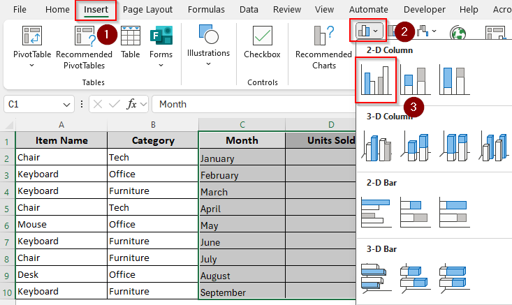
➤ To create a chart representing the months and sold units for each month, select the entire range from the month column and the sold units column.
➤ Go to the Insert tab and navigate to the Charts group.
➤ Choose a chart type that suits the best for your data type. As we’re working with time-based data, we chose a Clustered Column chart.
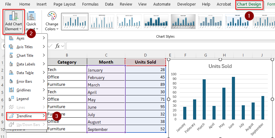
➤ To add a moving average trendline to your chart, go to the Chart Design tab and press the Add Chart Element button from the Chart Layouts group.
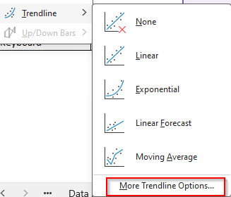
➤ Select Trendline from the menu and choose More Trendline Options.
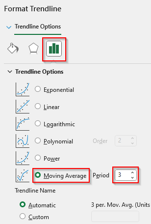
➤ As the Format Trendline pane appears, click on the Trendline Options icon >> Moving Average.
➤ In the Period box, set the number of periods. For example, we chose 3 to average every 3 data points.
➤ You can click the Fill & Line icon to format the trendline style, color, size, etc.
➤ Close the pane to see the result. You can change the averaging period and add more lines following the same steps.
Frequently Asked Questions
How is the running annual average calculated?
We calculate the running annual average by averaging only the latest 12 months (or 365 days) of data, dropping the oldest value as each new one is added. For this, use this formula:
=AVERAGE(D2:D13)
Here, cells D2:D13 contain 12 months of data. Change the range as needed. This formula gives you the first year’s data. As you add new data for the latest months, copy the formula down so the range shifts (e.g., D3:D14, D4:D15, etc.) to create the running annual average.
How to calculate an Excel rolling average based on date?
If your data has dates in column C and values in column D, you can use an AVERAGEIFS formula to dynamically average only the values within your desired date range. For example, to calculate a 30-day rolling average for the date in C2:
=AVERAGEIFS($D:$D, $C:$C, “>=” & C2-29, $C:$C, “<=” & C2)
This formula finds all dates from 29 days before to the current date and averages the corresponding values.
How to get the highest running average in Excel?
First, calculate your running averages in a separate column using a moving average formula. After that, insert the following formula with the MAX function to find the highest average:
=MAX(E2:E10)
Here, E2:E10 is the column containing your running averages. Replace the range according to your dataset.
Concluding Words
Depending on whether you want to smooth data, spot trends, or keep a cumulative track, you can calculate mainly 3 types of running averages, including cumulative, SMA, and WMA. While applying a formula, make sure you use the correct range for accurate results.
Keep in mind that in SMA calculation, a formula might return blanks or #N/A for the first few cells as they don’t have enough data to calculate the average for your specified period.