How to Calculate Average in Excel Excluding 0

While calculating average in Excel, including zeros affects the accuracy of the calculation as it usually lowers the average. It doesn’t add anything to the sum of values, but is counted as valid while adding the numerical values.

Therefore, you must exclude zeros to only count cells with meaningful data and get the actual results. For this, you can use the AVERAGEIF function which lets you average numbers based on a condition.

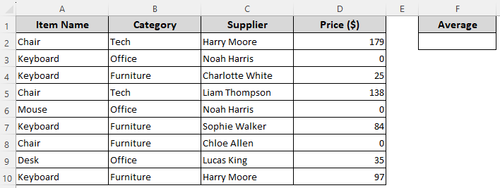
In our sample dataset, we have columns for product names, categories, supplier names, and prices. We’ll use the prices in Column D to calculate the average and put the value in cell F2. Here, cells D3, D6, and D8 contain a zero(0).

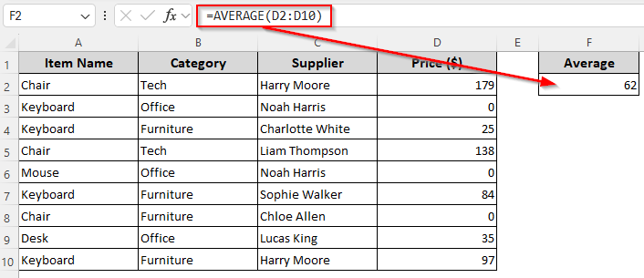
Below is the average when we include cells with zeros in the calculation:

To ignore the zeros, we can use the AVERAGEIF or AVERAGEIFS function. While the AVERAGEIF function calculates the average of cells that meet one condition, the AVERAGEIFS function averages cells meeting multiple conditions. We can use these functions to avoid cells containing zeros in the following way:

➤ In a cell where you want to put the average value, enter any of the following formulas:

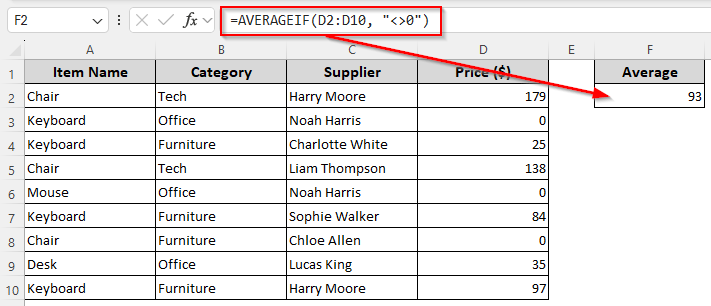
Average with One Condition

➤ For excluding zeros only, use this formula:

➤ Here, D2:D10 is the range of numbers, and “<>0” is our condition meaning not equal to zero. Change the range according to your dataset.
➤ Press Enter.

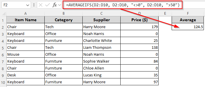
Average with Multiple Conditions

➤ If you have more than one condition like excluding zeros and only averaging numbers above 50, use this formula:

➤ Change the range D2:D10 and condition “>50” as per your requirements.
➤ Click Enter.

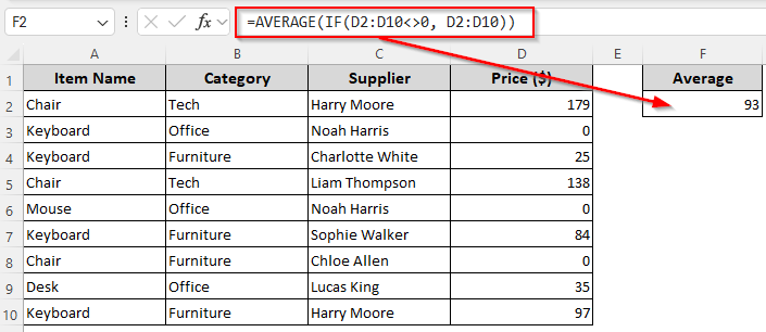
For older Excel versions without AVERAGEIF, we can combine the AVERAGE and IF functions to exclude zeros. In our formula, the IF function will check for numbers not equal to zero(0). Those numbers are passed to AVERAGE for further calculation. Below are the details:

➤ Select a cell for the average value and insert the following formula:

➤ Replace D2:D10 with the actual source range containing the values to average in your dataset.
➤ As this is an array formula, you must press  Ctrl  +  Shift  +  Enter  in Excel 2016 or older versions. For newer versions, click  Enter  .

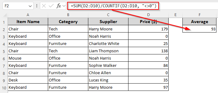
Here, we’ll take a mathematical approach that divides the sum by the count of non-zero values. In our formula, the COUNTIF will count only cells that are not zero and the SUM function will add all the numbers within a range.

➤ Choose a cell to return the average value and enter this formula:

➤ Replace the range D2:D10 as required.
➤ Press Enter.

With the FILTER function, you can extract specific data from a range based on a condition. We’ll apply a condition to filter numbers that aren’t zero and use the AVERAGE function for further calculation. Let’s get to the steps:

➤ In a cell to return the average value, type the following formula:

➤ Change the range D2:D10 as needed.
➤ Press Enter.

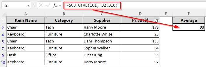
Even if you don’t have the FILTER function, you can manually filter out zeros and then apply the SUBTOTAL function to calculate the average using the filtered data. Here’s how:

➤ Select your data range (including the header) and go to the Data tab. Select Filter from the Sort & Filter group.
➤ As Excel adds a filter drop-down on the column heading, click the filter drop-down and uncheck 0.
➤ When the filtered data without the zeros is displayed, enter the following formula in a cell to get the average:

➤ Change the data range D2:D10 according to your dataset.
➤ Press Ok to calculate the average.

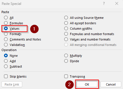
➤ Now, copy the average using  Ctrl  +  C  and right-click on the same cell. Choose Paste Special from the menu.

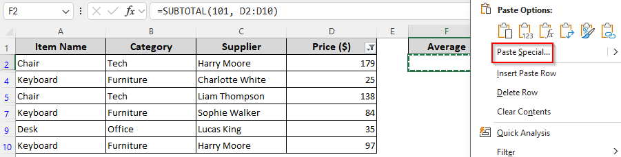
➤ From the Paste Special dialog box, select Values and click Ok.

➤ To bring back your original data, go to the Data tab >> Filter.

The AGGREGATE function ignores errors and hidden rows, but it doesn’t have a built-in ignore zeros option. So, to exclude zeros, we’ll use the IF function to create an array where zero values are turned into cause a #N/A errors so that AGGREGATE ignores them while calculating the average. For this, follow these steps:

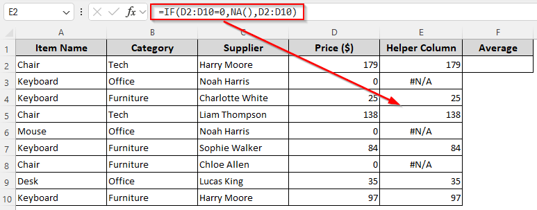
➤ Create a helper column and the following formula in its first cell:

➤ Change the range D2:D10 as required.
➤ For Excel 365/2021, just press  Enter  . In older Excel versions, press  Ctrl  +  Shift  +  Enter  and Excel will return an array.

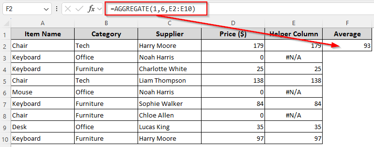
➤ Now, choose a cell to put the average and insert this formula:

➤ Here, function number 1 calculates the average, and function 6 ignores errors in the returned array range E2:E10.
➤ Replace the range D2:D10 according to your dataset.
➤ Click Enter.

Frequently Asked Questions

How to average without zeros and negative numbers?

To exclude zeros, negative values, blanks, and texts from the average calculation, you can use AVERAGEIF with a condition. For this, insert the following formula:
=AVERAGEIF(D2:D10, “>0”)
This formula only includes values greater than 0. Change the range D2:D10 as needed and press Enter.

How do I ignore errors in the Excel average?

We can ignore errors while calculating the average using the AGGREGATE function. Insert the following formula:
=AGGREGATE(1, 6, D2:D10)
Here, function code 1 calculates the average, and function code 6 ignores errors. Replace D2:D10 with your original range and click Ok.

How do you ignore divide by zero in the Excel average?

Divide-by-zero errors happen when the denominator is zero. To avoid it using the IFERROR function, use this formula:
=IFERROR(SUM(D2:D10)/COUNTIF(D2:D10,”<>0″), “”)|
Change D2:D10 with your source range and press Enter. If COUNTIF finds no non-zero numbers, the denominator would be 0, but IFERROR will return a blank instead of a #DIV/0! error.

Concluding Words

All the above-mentioned functions exclude zero in the average calculation when used with correct conditions. If you want to work manually, you can filter rows containing zeros.

However, for longer datasets, the AVERAGEIF method is the simplest for basic needs, while the AVERAGEIFS function offers the most flexibility for complex datasets. Choose the method that best fits your specific data structure and requirements.