How to Combine SUMIF with INDEX-MATCH Formula in Excel

In the INDEX-MATCH formula, MATCH finds the relative position of a lookup value in a range and INDEX returns a match from a specified row and column in a range based on that value. The SUMIF function adds cells that meet a single criterion you specify.

When combined, they allow you to perform conditional summations with dynamic ranges, multiple criteria, and advanced lookups. This is incredibly useful when your sum range needs to change based on another lookup.

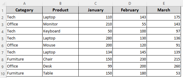
Our sample dataset has 5 columns for product categories (Column A), names (Column B), and monthly sales figures for January (Column C), February (Column D), and March (Column E).

Although the SUMIF function requires you to manually specify the sum range, you can make it dynamic by combining it with INDEX-MATCH. Here, we’ll look for Laptop and get the sum of its total sales in January. Below are the steps:

Formula with Lookup Texts

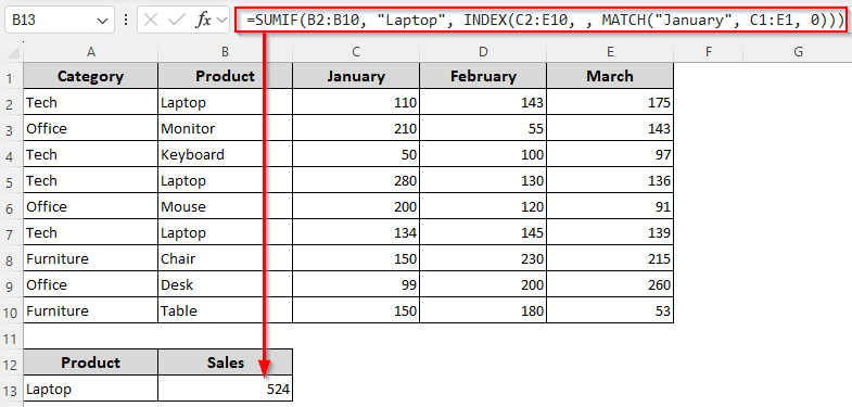
➤ If you want to hardcode the lookup values in your formula, insert this formula in a cell where you want the summed value:

➤ Here, our lookup value is Laptop and B2:B10 is the product list (criteria range) containing the value Laptop. C2:E10 is our return range containing the prices. We want to sum up the value from the return column January and it’s in the range C1:E1. Replace these values according to your source data.
➤ Press Enter.

Formula with Lookup Cell References

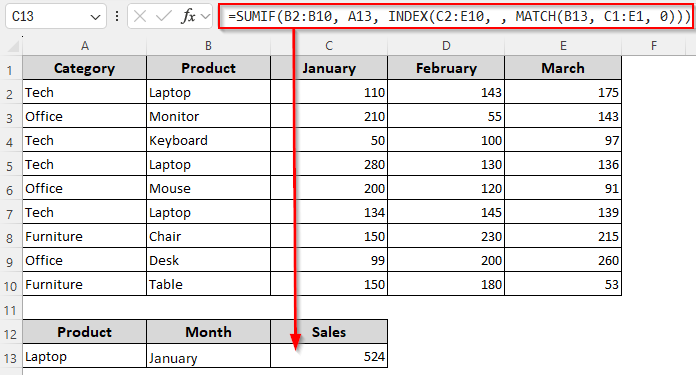
➤ To lookup with cell references, first, enter the criteria Laptop in cell A13. Now, enter the lookup value January in B13. We’ll insert the following formula in C13 to return the total sales in it:

➤ Change the ranges and cell references as needed.
➤ Click Enter.

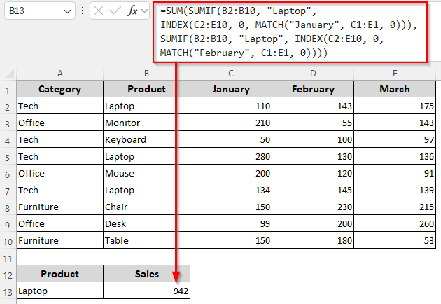
As SUMIF only works with a single criterion, we use the SUMIFS function for multiple criteria in modern Excel. However, There’s only one way to do a conditional sum with multiple criteria across different row/column dimensions. To sum the sales for Laptop in the months of January and February, follow these steps:

➤ In a cell where you want the summed value, enter the following formula:

➤ Change the criteria ranges B2:B10 and C1:E1, return range C2:E10, and criteria values Laptop, January, and February as needed.
➤ Press Enter.

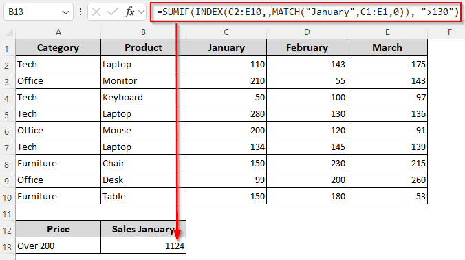
Numeric conditions like greater than, less than, equal to, not equal, etc., work perfectly with SUMIF and INDEX-MATCH. However, SUMIF alone cannot handle two conditions (product and numeric) at once. In this example, we’ll sum the sales in January (Column C) only if they are greater than 130. Here’s how:

➤ Enter the following formula in the cell where you want the summed value:

➤ Depending on your dataset, replace the criteria January, criteria range C1:E1, return range C2:E10, and numeric condition >130.
➤ Click Enter.

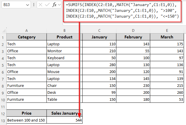
Use this method to filter the data you want to sum based on two numeric conditions. For example, here we’ll sum the sales in January only if they are between 100 and 150. Let’s get to the steps:

➤ Select a cell to return the summed value and enter the following formula in it:

➤ You can change the criteria range C1:E1, return range C2:E10, lookup value January, and the numeric conditions >100 and <=150 according to your source data.
➤ Press Enter.

Here, our lookup value itself is a conditional sum. With our formula, we’ll find a product whose total sales across months meet a certain threshold (over 500). Let’s get into the details:

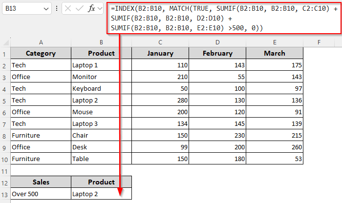
➤ To find the name of the first product (from Column B) whose total sales (January+February+March) exceed 500, enter this formula:

➤ Depending on your source data, change the lookup range B2:B10, the return ranges C2:C10, D2:D10, and E2:E10, and the numeric condition >500.
➤ For Excel 365/2021, press  Enter  . If you’re using an older version, click  Ctrl  +  Shift  +  Enter  .

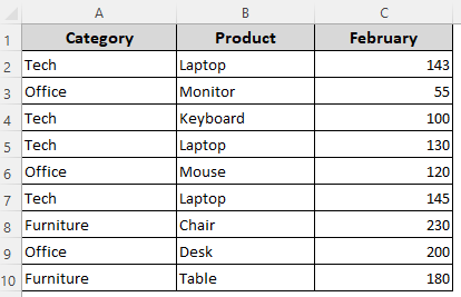
For multi-sheet summation, we created a new Sales sheet where we insert the name of the tab from which we’ll extract the values to sum. We have 3 tabs named January, February, and March to represent the sales for the months.

Each sheet has 3 columns with product categories (Column A), names (Column B) and monthly sales data (Column C). To sum the sales for a specific product (Laptop) from the correct sheet (February) dynamically, follow these steps:

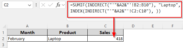
➤ Enter the sheet name February in cell A2 of the Sales tab. Insert this formula in a cell where you want to return the total price for Laptop from the February tab.

➤ Here, A2 is the cell containing the lookup sheet name, B2:B10 is the criteria range containing the criteria product Laptop, and C2:C10 is the return range containing the sales numbers to sum. Replace them as required.
➤ Click Enter.

Frequently Asked Questions

Can I use SUMIFS with INDEX MATCH for multiple criteria?

Yes, you can combine SUMIFS with INDEX-MATCH to dynamically select ranges or columns. To sum sales for a product in a specific month, use this formula:
=SUMIFS(INDEX(C2:E10,,MATCH(“February”,C1:E1,0)), B2:B10, “Laptop”)
You can replace the criteria February and Laptop, criteria ranges C1:E1 and B2:B10, and return range C2:E10 and click Enter to get the result.

Why is SUMPRODUCT better than SUMIF?

While SUMIF only allows one condition at a time, SUMPRODUCT can handle multiple criteria, numeric conditions, and complex calculations in a single formula. For example, to sum sales of Laptop in February if sales >150, you can use the following formula:
=SUMPRODUCT((B2:B10=”Laptop”)*(D2:D10>150)*D2:D10)
➤ Here, B2:B10 is the lookup range containing the lookup value Laptop. D2:D10 contains the sales data for February month. Change the values and press Enter to get the total. Unfortunately, you can’t do it with a single SUMIF.

How to sum all matching values in Excel?

You can use SUMIF to add all values that meet a specific condition. If you want to sum all sales for Laptop, use:
=SUMIF(B2:B10, “Laptop”, C2:C10)
If Laptop appears multiple times in the lookup range B2:B10, SUMIF adds all matching rows from the return range C2:C10. Change these values if needed and click Enter to get the sum.

Concluding Words

Apart from the functions mentioned above, the combination of SUMIF and INDEX-MATCH also works with other Excel functions like IFERROR, which replaces errors with your defined value when the lookup criteria isn’t matched.

For multiple criteria and more flexibility, you can use SUMIFS or SUMPRODUCTS instead of SUMIF. Pair them with the INDEX-MATCH formula to make the ranges and criteria dynamic.