An expense report lists all the money you have spent over a certain period. Businesses use it to track expenses, while individuals use it to manage their personal budgets. Excel is the perfect tool for creating this report because it can do all the calculations easily. In this article, we will show you how to create a dynamic Expense report in Excel.
To create an expense report in Excel, here is one simple solution using the Excel Table and Data Validation feature.
➤ Start by removing default Gridlines for a cleaner, document-like appearance.
➤ Use Merge & Center and Cell Styles to create the title.
➤ Convert data range into an Excel Table.
➤ Apply Data Validation to the Expense and Category columns for error-free data entry.
➤ Use a simple subtraction formula in the Due Amount column to get the due amount result.
➤ Activate the Total Row feature to calculate the total expenses and thus create a complete expense report in Excel.
Steps to Create an Expense Report in Excel
Here, we will explain how to create an Expense report in Excel with a step-by-step process. We will break down the process into four simple steps: designing the layout, setting up data validation, and calculating the final results.
Step 1: Designing the Layout
The first step involves setting up the structure and main components of the expense report.
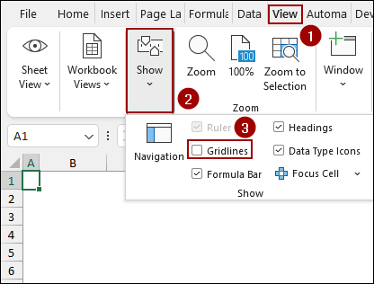
Simply, open a new Excel sheet and remove the default gridlines to make the report look more professional.
➤ Go to the View tab, select the Show group, and uncheck the Gridlines option.
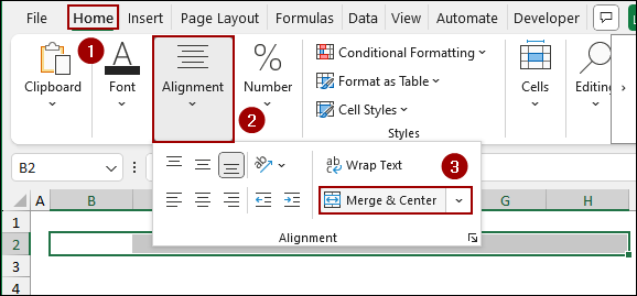
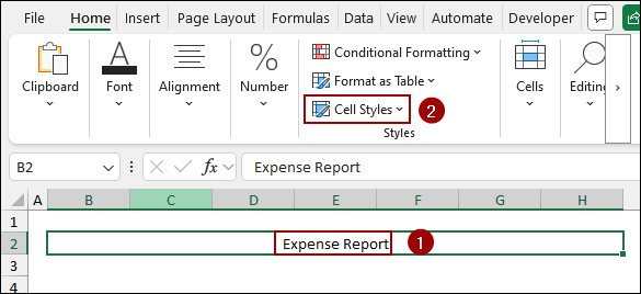
➤ Select the cells for the main title (e.g., A2:G2), go to the Home tab, select Alignment, and click Merge & Center.
➤Type “Expense Report” into the merged cell.
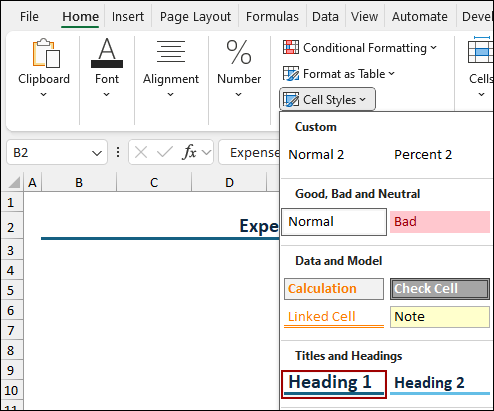
➤ With the title cell selected, go back to the Home tab and, in the Styles group, click Cell Styles.
This feature allows you to quickly apply a professional, pre-set formatting.
➤ Choose a style like Heading 1 from the menu.
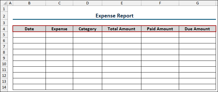
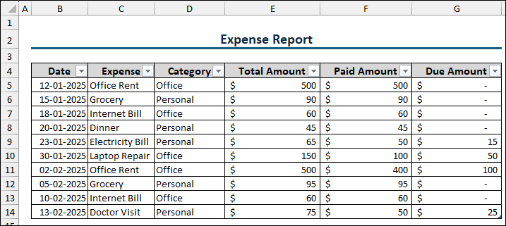
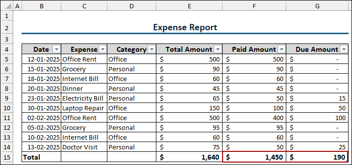
➤ Next, set up the column headers for your expense data starting from row 4: Date, Expense, Category, Total Amount, Paid Amount, and Due Amount.
➤ Apply borders to the cells to clearly define the data entry area.
➤ Select the entire range of data, including the headers (e.g., B4:G14), and go to the Insert tab, click Tables to convert the range into an Excel Table.
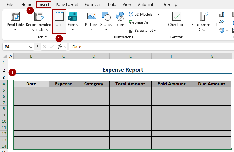
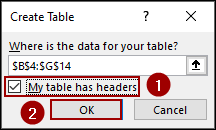
➤ In the Create Table dialog box, ensure the correct data range is selected and that the My table has headers box is checked, and click OK.
Thus, the table will be created. This is crucial for enabling the dynamic features of the table.
Step 2: Setting Up Data Validation
To prevent data entry errors and ensure consistency, we will create dynamic drop-down lists for key columns.
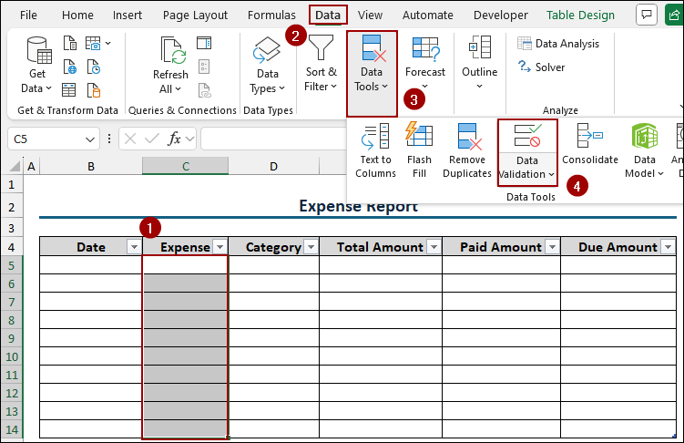
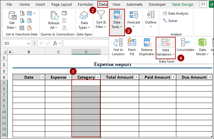
➤ Select all the cells under the Expense column (e.g., C5:C14) where you want the drop-down list to appear.
➤ Go to the Data tab, click the Data Tools group, and select Data Validation.
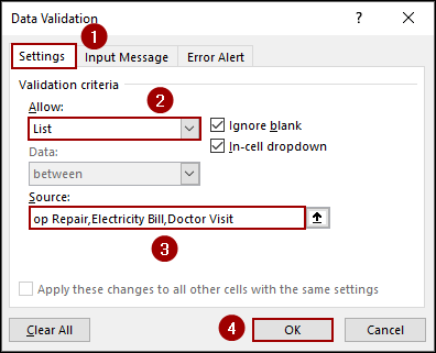
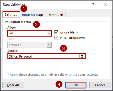
➤ In the Data Validation dialog box, navigate to the Settings tab.
➤ From the Allow drop-down menu, choose List.
➤ In the Source box, enter your expense list, separated by commas (e.g., Office Repair, Electricity Bill, Doctor Visit, etc.).
➤ Click OK.
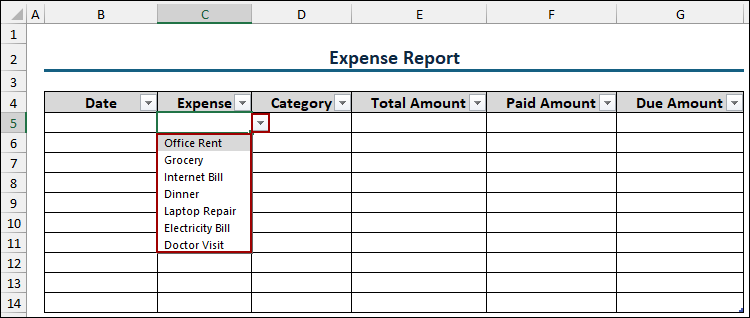
A drop-down arrow will now appear in each cell of the Expense column, displaying your list of choices.
Repeat the Data Validation process for the Category column (e.g., D5:D14).
➤ Select the column range and go back to Data Validation.
➤ On the Settings tab, choose List again and enter your categories in the Source box, separated by commas (e.g., Office, Personal).
➤ Click OK.
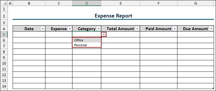
The Category column now also has a drop-down list, limiting entries to either “Office” or “Personal”.
Step 3: Calculating Final Result
We will now implement a simple formula in the Due Amount column. Since we used an official Excel Table, this formula will automatically apply to every row.
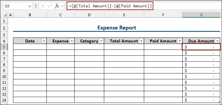
➤ Click on the first cell in the Due Amount column (G5).
➤ Enter the formula to calculate the difference between the total expense and the paid amount.
=[@[Total Amount]]-[@[Paid Amount]]
The use of structured references (like [@[Total Amount]]) allows the table to manage the formula dynamically.
➤ Hit ENTER.
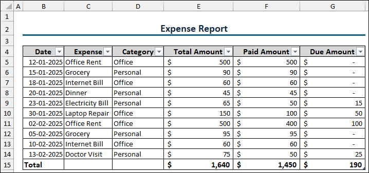
Excel’s table feature instantly fills this formula down the entire column. Now, inserting expense data (Date, Expense, Category, Total Amount, Paid Amount), the Due Amount will be calculated automatically.
Here, we have inserted some expenses for office and personal.
Now, we will use the table’s summary feature and use the built-in filters for analysis.
➤ Click anywhere inside the table.
This will activate the Table Design tab on the ribbon.
➤ In the Table Style Options group, check the Total Row option.
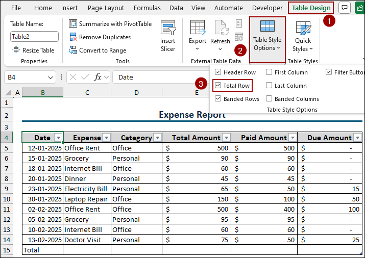
A new Total row will appear at the bottom of your table.
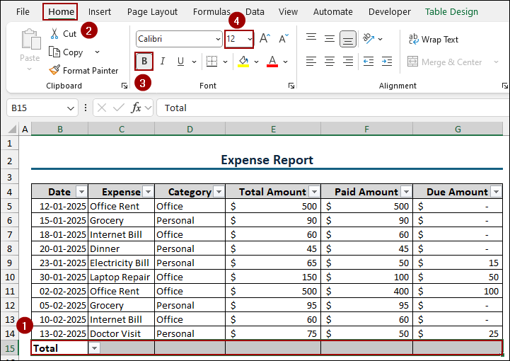
➤ Choose the cells in the Total Amount column within this new row.
➤ Change the Font to Bold and increase Font Size to 12.
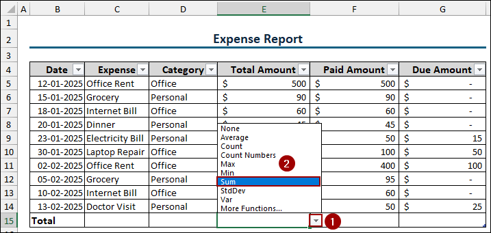
➤ Click the cell in the Total Amount column within this new row.
A drop-down arrow will appear in the Total row cell.
➤ Click this arrow to open the summary options.
➤ Select Sum from the drop-down list.
This will instantly calculate the sum of all values in the Total Amount column.
Repeat this for the Paid Amount and Due Amount columns to get the final totals. Finally, we have successfully created an expense report in Excel.
➤ To quickly analyze expenses by category, click the filter arrow next to the Category column header.
➤ Uncheck the Select All box, and then check only the category you wish to view (e.g., Office).
➤ Click OK.
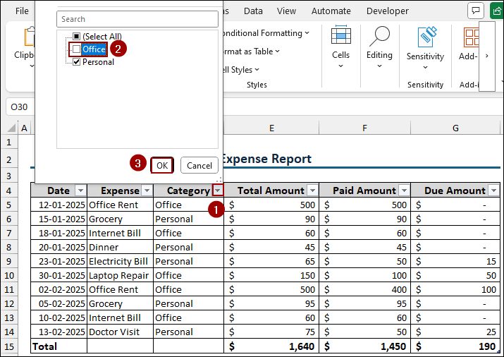
As a result, your expense report now only displays the selected category’s data, and the Total Row summary automatically updates to reflect only the filtered data.

Frequently Asked Questions
How can I protect my expense report from accidental changes?
You can lock specific cells or the entire sheet. Go to the Review tab, click Protect Sheet, and set a password. This prevents accidental changes to your formulas and table structure.
Is it better to use VLOOKUP or a drop-down list for categories?
A simple Data Validation (drop-down list) is faster for a simple report. If you have hundreds of categories, the VLOOKUP function is a better choice for pulling data automatically based on the selected category name.
How do I add more rows to my expense report table?
As the report is converted to an Excel Table, you can simply click on the last cell (the one before the Total row) and press the TAB key. A new row will automatically be created, and all formulas will extend to it.
Concluding Words
Above, we have covered all the steps to create a dynamic expense report in Excel. The key feature involves utilizing the Excel Table feature and the Data Validation to create a system that automates calculations. If you have any further questions, please feel free to share them in the comments section below.