One of the most popular methods for determining how an independent variable relates to a dependent variable is linear regression. Whether you’re examining scientific patterns, forecasting stock prices, or evaluating sales data, Excel has built in tools to easily perform linear regression. In this tutorial, you will learn about linear regression and how to do linear regression in Excel using Add-ins, functions, and charts.
➤ Linear regression models the relationship between independent and dependent variables by fitting a straight line. ➤ Regression Graph: In this article, we’ll learn how to do linear regression in Excel with Data Analysis ToolPak, formulas, and charts. Additionally, we’ll discuss and interpret the results of the linear regression analysis.
➤ Enable Data Analysis: File >> Options >> Excel Add-ins >> Data Analysis.
➤ Regression: Data tab >> Data Analysis >> Regression >> Input Y range >> Input X range >> Labels >> Output range >> OK.
➤ Formulas:=INTERCEPT(known_ys,known_xs)=SLOPE(known_ys,known_xs)=CORREL(array1, array2)=LINEST(known_ys, [knownn_xs])
What Is Simple Linear Regression?
Linear regression models the relationship between an independent variable (predictor) and a dependent variable (outcome) by fitting a line of best fit through the data.
Simply put, a linear regression model measures how far the actual data points are from the straight line. It uses the sum of squares approach to calculate these distances. The goal is to find the line that minimizes these distances; in other words, the line that best fits the data.
The general equation formula for linear regression is:
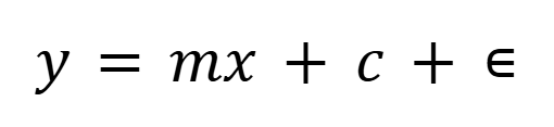
where,
- y is the dependent variable
- x is the independent variable
- m is the gradient or the change in y for each unit change in x
- c is the y intercept or the point where the regression line crosses the y axis
- ∊ is the error term representing the difference between the actual and predicted values.
In the real world, the independent variable (predictor) is never entirely accurate; therefore, an error term (∊) is always present in the linear regression equation. However, Excel calculates this error term in the background, so when performing linear regression in Excel, just determine the coefficients of m and c. The general equation reduces to:
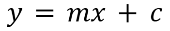
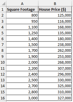
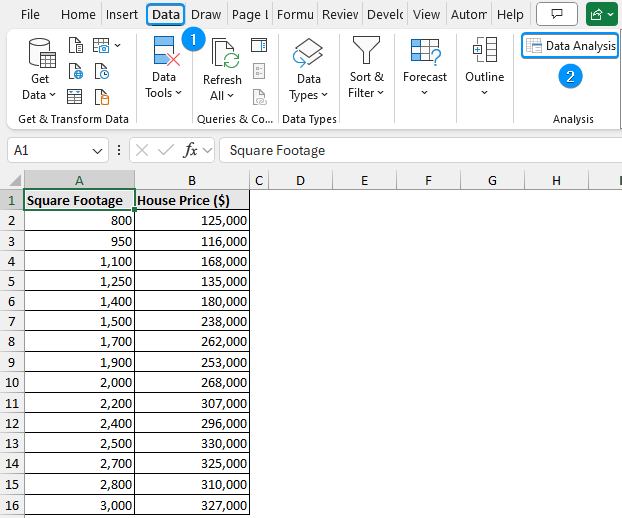
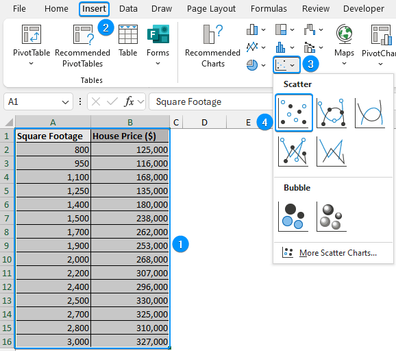
Let’s assume you are a real estate analyst who wants to predict house prices based on the square footage. In this case, there are 15 observations with different square footage and corresponding house prices in US Dollars. The square footage in column A is the independent variable (predictor), while the house prices in column B represent the dependent variable (outcome). By performing a linear regression, you can determine the gradient (m) and y intercept (c) to construct a linear equation like this:
House prices = Square footage × (gradient) + y intercept
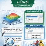
This simple linear regression model will help you forecast house prices based on the square footage. There are three methods for performing linear regression in Excel. Let’s look at the detailed steps for each method.
Linear Regression in Excel with Data Analysis ToolPak
Excel’s Data Analysis ToolPak provides a comprehensive method for performing linear regression with detailed statistical results. It is available in all versions of Excel, but you need to activate this tool. Just follow along.
Steps:
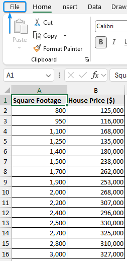
➤ Click on the File tab.
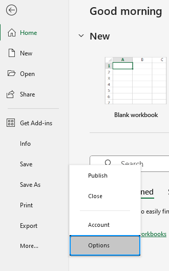
➤ Select Options. You can also use the shortcut Alt + F + T to open Excel Options.
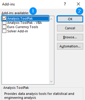
➤ Select Add-ins >> Choose Excel Add-ins from the dropdown >> Go.
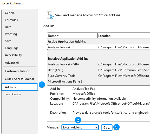
➤ Check the Analysis ToolPak option >> OK.
The Data Analysis ToolPak will be available in the Data tab whenever you open a new workbook.
➤ Go to the Data tab >> Click Data Analysis.
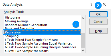
➤ Select Regression >> OK.
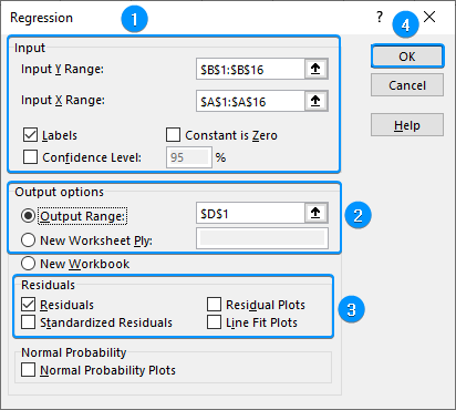
➤ Select Input Y Range (B1:B16) and Input X Range (A1:A16).
➤ Check the Labels option. Choose the Output Range (D1).
➤ Select the Residuals option >> OK.
Interpretation of Linear Regression Results
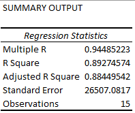
Summary Output:
➥ Multiple R: The correlation coefficient signifies the strength and direction of the relationship between two variables. It ranges from -1 to +1. A +1 shows a perfectly positive correlation while -1 shows a perfectly negative correlation. A 0 indicates no meaningful correlation.
➥ R Square: The coefficient of determination measures the proportion of variance in the dependent variable that is explained by the independent variable. For example, 89.2% of the variation in house prices can be explained by the square footage variable.
➥ Adjusted R Square: The adjusted R square value based on the number of independent variables. It is useful in the case of multiple regression.
➥ Standard Error: The average distance the observations are located from the regression line. For example, on average the observed values are located 26,507.08 units from the regression line.
➥ Observations: The number of observations.
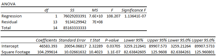
ANOVA:
- df: Degrees of freedom.
- SS: The sum of squares.
- MS: The mean sum of squares.
- F: The F statistic.
- Significance F: The P value of the F statistic.
The significance F reveals whether the results are reliable. The regression model is reliable if the significance F value is less than the significance level (0.05). If the significance F is greater than the significance level, we must choose a different independent variable.
Regression Coefficients:
The coefficient indicates the average change in the dependent variable for each unit change in the independent variable. For example, the house price increased by $104.30 for each unit increase in the square footage.
The coefficients can be used to make a regression equation like this:
House price = Square footage coefficient × Square footage + Intercept
Replacing the values from the regression output:
House price = 104.30 × Square footage + 46583.4
Plug the square footage (x) value to calculate the house price based on the regression model.
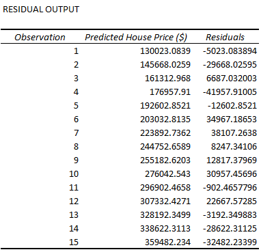
Residual Output:
The difference between the actual value and the value predicted by the regression model.
Notice the house price estimated by the regression model is $130,023, whereas the actual value in cell B2 is $125,000. Subtracting the residual from the predicted house price gives the actual house price.
Simple Linear Regression with Excel Functions
You can use Excel functions to perform linear regression analysis.
Steps:
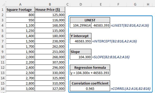
➤ The LINEST function uses the least squares method to fit a straight line that explains the relationship between the two variables. The LINEST function returns an array of values, so press the Ctrl + Shift + Enter keys for earlier versions of Excel. In newer versions, just press Enter .
=LINEST(B2:B16,A2:A16)
To avoid array formulas, we can use other functions to construct a linear regression equation.
➤ The INTERCEPT function to calculate the y intercept.
=INTERCEPT(B2:B16,A2:A16)
➤ The SLOPE function calculates the gradient of the line.
=SLOPE(B2:B16,A2:A16)
➤ The CORREL function calculates the correlation coefficient between two variables.
=CORREL(A2:A16,B2:B16)
➤ The regression formula is y=mx + c, where m is the slope and c is the y intercept. Plug the x value into the formula to calculate the y value.
=104.300x+46583.393
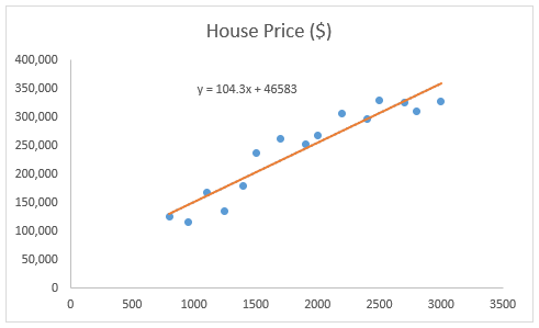
Linear Regression Graph in Excel (Least Squares Regression Line)
A linear regression graph is a visual representation of the relationship between two variables using the least squares regression line. This line best fits the data by minimizing the squared differences between actual and predicted values. By adding the least squares regression line, you can display both the equation of the line and the R² value directly on the chart for easy interpretation.
Steps:
➤ Select the entire dataset (A1:B16) >> Insert >> Insert Scatter or Bubble Chart >> Scatter.
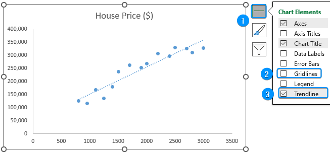
➤ Click on Chart Elements >> Remove Gridlines >> Check Trendline to add the least squares regression line.
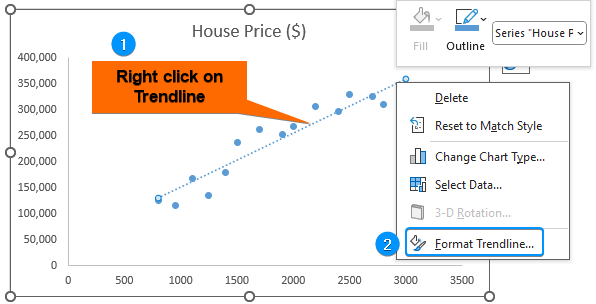
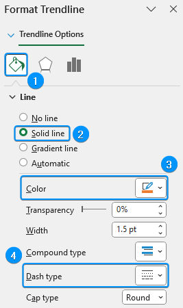
➤ Right click on the Trendline >> Format Trendline.
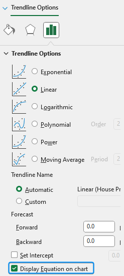
➤ Enable the Display Equation on chart option.
➤ In the Fill & Line tab, Solid Line >> Color (Orange, Accent 2) >> Dash type (Solid).
➤ You can plug in a value of x (Square footage) to predict the value of y (House price).
Frequently Asked Questions
How do you run a linear regression in Excel?
Select data >> Data tab >> Data Analysis >> Regression >> Input Y range >> Input X range >> Labels >> Output range >> OK.
Or,
Y intercept: =INTERCEPT(known_ys,known_xs)
Slope: =SLOPE(known_ys,known_xs)
CORREL: =CORREL(array1, array2)
When to use simple linear regression?
Simple linear regression should be used when there is one independent (predictor) and one dependent (outcome) variable. If there are multiple independent variables and one dependent variable, perform multiple linear regression instead.
What do R squared and Adjusted R squared mean in regression analysis?
R squared indicates the percentage of variance in the dependent variable that is explained by the independent variable. Adjusted R squared adjusts for the number of independent variables, providing a more accurate measure of model fit, especially in multiple regression.
How can I interpret the regression output in Excel?
Key metrics:
- R squared: A value of 1 means the model perfectly explains all the variability while 0 indicates no relationship.
- P value: Check the statistical significance. The model is reliable if the P value is less than the significance level.
- Correlation coefficient: Indicates the relationship strength and direction.
Can I do multiple linear regression in Excel?
Yes, using the Data Analysis Toolpak. When setting up the regression, select multiple columns for your independent variables.
Wrapping Up
In this tutorial, we’ve learned about linear regression, how to do linear regression in Excel with Data Analysis ToolPak and functions. Moreover, we’ve plotted a Scatter chart, fitted a regression line, and obtained the equation of the regression line. Feel free to download the practice file and let us know which method you like the most.