
Basically, the SUMIF function in Excel works with specific values or conditions, not cell colors. In fact, Excel doesn’t offer any function that can sum values based on cell colors. So, this is one of the most frustrating limitations we usually face while working with visually formatted worksheets.
But don’t worry. There are still some tricky ways to sum values by cell color in excel like GET.CELL, FILTER + SUBTOTAL functions or even VBA. Let’s walk through these methods step-by-step.
To begin with, let’s explore a quick Excel SUMIF cell color formula.
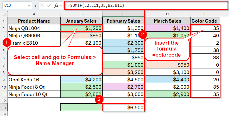
➤ Choose cell B2.
➤ Go to Formulas > Name Manager.
➤ Fill the Name and Refers to sections and press Ok.
➤ In cell E2, insert the Name with an equal (=) sign before the name to get the Color Code.
➤ Now insert the following formula in cell C13:
=SUMIF(E2:E11,35,B2:B11)
➤ Press Enter and here’s the result.
Now, let’s dive deeper into this tutorial and explore more of these methods.
Overview of the SUMIF Function in Excel
As we mentioned earlier, the SUMIF function adds values in a range that meet a single criterion you set. Normally, that criterion could be a number, text, or date, but not a color.
Syntax:
SUMIF(range, criteria, [sum_range])
➤ range → The cells you check for your condition.
➤ criteria → The condition to match.
➤ sum_range → (Optional) The actual cells to sum.
Example:
=SUMIF(B2:B11, ">1000", C2:C11)
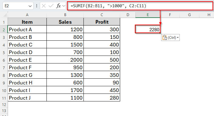
This sums values in C2:C11 where the corresponding value in B2:B11 is greater than 1000.
Using Excel SUMIF Function with Cell Color Code (GET.CELL)
If you want to use specifically the SUMIF function to sum values by the cell color, this would be the only method you can try. This method is not as elegant or popular as the other methods we’ll discuss later, but it’s the only way that will allow you to use the SUMIF function.
Typically, the GET.CELL is quite different from other regular Excel functions. Because this function is a built-in function in Excel that retrieves information about the formatting, location or contents of a cell. But it cannot be directly referred to the worksheet.
However, in this method, we have to enable the GET.CELL function which can generate the color index value of the colored cells in a dataset. Then, we can simply apply a SUMIF formula to get the sum of cells with a specific color.
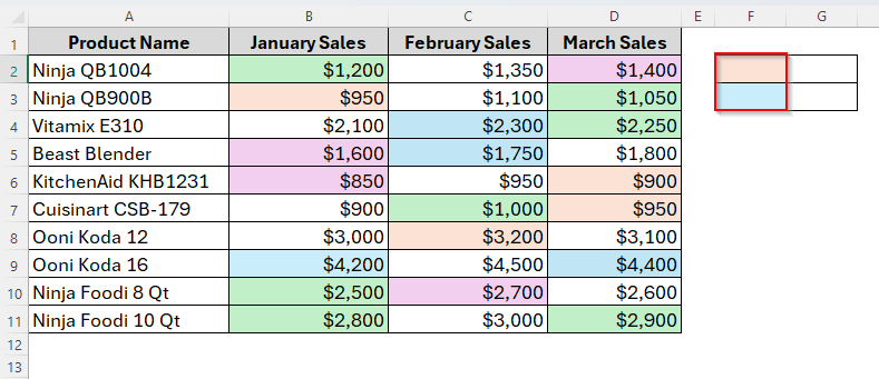
For this, today we have a dataset of some Product Names and their monthly basis Sales. Here, you can see multiple colors in the background of some cells.
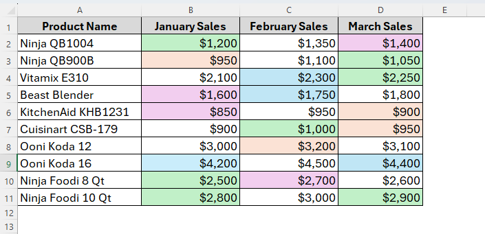
So, let’s assume we’ll count the total amount of the cells with the color Green from Column B and here, how it goes.
Steps:
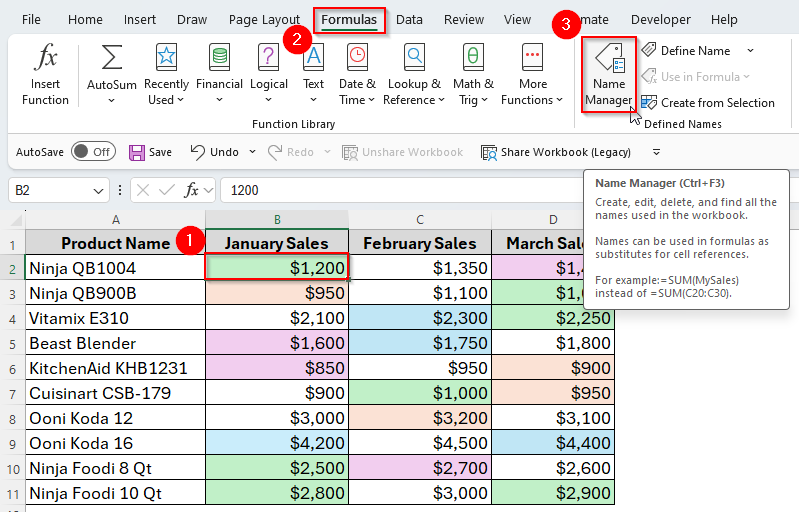
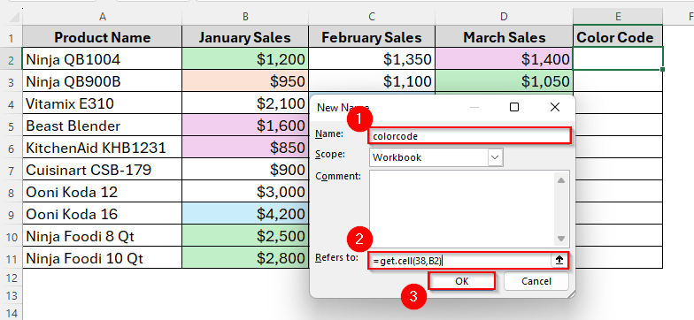
➤ Click on the cell B2 and go to the Formulas > Name Manager in the Ribbon. Alternatively, you can also tap Ctrl + F3 to open the Name Manager dialogue box.
➤ Now, under the New option from the Name Manager dialogue box, enter the Name to colorcode and Refers to = get.cell(38,B2).
Note:
Here, 38 is the first argument inside the function which refers to the specific characteristic we want to evaluate in a cell. As we want to evaluate the background color, the code we used is 38.
In fact, there are multiple codes available you can enter in here. For example, we could be evaluating whether or not there is a top border or a bottom border or other ways we’ve formatted the cells. Then, the other argument we entered is which cell is being evaluated. We choose B2, as we want to sum cells with Green color from the Column B.
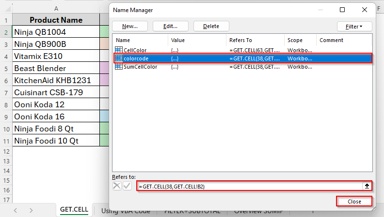
➤ Click Ok and Close the dialogue box.
➤ Now in cell E2, insert the following formula:
=colorcode
This is what we actually entered in the Name section of the Name Manager dialogue box. You can give it any kind of name, but make sure to insert the same name in this formula.
➤ Press Enter and we’ll get the color index of the cells from column B.
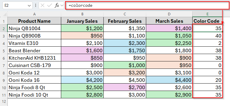
So, as you can see in the image above, the color code for the Green color is 35. Similarly, we’ve got multiple color codes for different colors like 40 for Bisque, 38 for Pink, 20 for Blue and 0 for White.
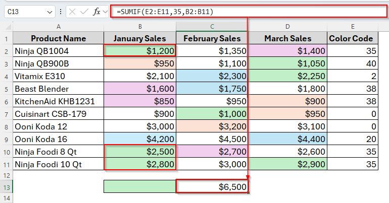
➤ Once we have the color code, insert the following formula in cell C13:
=SUMIF(E2:E11,35,B2:B11)
➤ Hit Enter and we’ll get the total sum of the values of cells with Green color in column B.
Alternatives to SUMIF Function to Sum by Cell Color in Excel
Though the GET.CELL function allows you to use the SUMIF function, this method is a little bit of a hassle while there are some other simple ways to sum values by cell color. For example, you can use a VBA code or apply the FILTER + SUBTOTAL functions instead. These are pretty much straightforward than the GET.CELL function.
Using VBA Code to Sum By Cell Color
As there’s no built-in functions or formulas to sum by cell color in excel, you can create your own formula by using VBA code. With VBA, a User-Defined Function (UDF) can be created and it will do all the work in the back end. Then, you can use the UDF like any other Excel function in your worksheet.
For example, now we’ll sum the values of cells colored Bisque and Blue from the same dataset. So, let’s see how it works.
Steps:
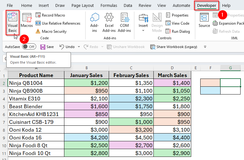
➤ To begin with, insert four blank cells in the worksheet and choose two specific colors from the dataset. As you can see in the image below, we’ve chosen the Bisque and Blue color in cell F2 and F3 respectively.
➤ Now, go to the Developer > Visual Basic from the Ribbon to open the Visual Basic Application.
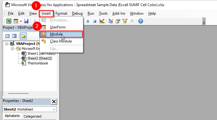
➤ Then, click on Insert and select Module.
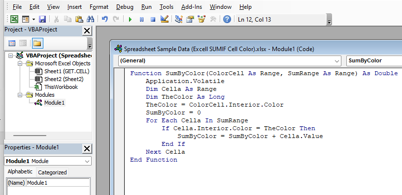
➤ Now, in the Visual Basic Editor, just copy and paste the following VBA code.
Function SumByColor(ColorCell As Range, SumRange As Range) As Double
    Application.Volatile
    Dim Cella As Range
    Dim TheColor As Long
    TheColor = ColorCell.Interior.Color
    SumByColor = 0
    For Each Cella In SumRange
        If Cella.Interior.Color = TheColor Then
            SumByColor = SumByColor + Cella.Value
        End If
    Next Cella
End Function
➤ Once you paste the code, it will look as follows.
➤ After that, close the Visual Basic Editor and go back to your worksheet.
➤ Now in cell G2, type the following formula:
=SumByColor(F2, B2:D11)
➤ Tap Enter and drag the formula down to cell G3. Now you’ll get the total sales amount from the cell colored Bisque and Blue.
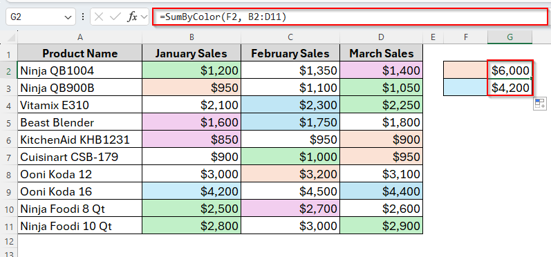
You can also add some more cells for other colors to sum values. All you need to do is just copy the formula down to the end using the AutoFill Handle.
Combining FILTER & SUBTOTAL Functions
This would be the simplest and easiest one among all these methods. Personally, I also prefer this method to sum values by cell color in Excel. Unlike the previous two methods, it goes through a few simple steps and doesn’t require any code or something.
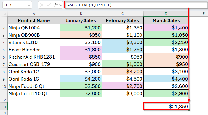
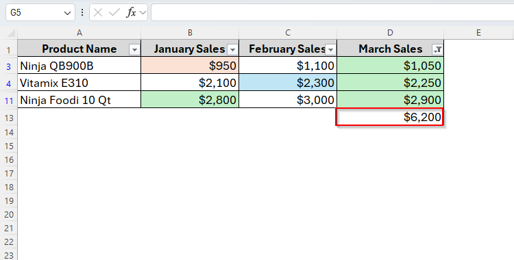
All it requires is just to count the total of all cells of the column using the SUBTOTAL function and then filter the cells with a specific color by the FILTER function. Now let’s sum the values of cells with the color Green from the Column D. To do so, below are the steps to follow.
Steps:
➤ Click on Cell D13 and insert the formula as follows:
=SUBTOTAL(9,D2:D11)
➤ Press Enter. Here we get the total sum of the values from the Column D.
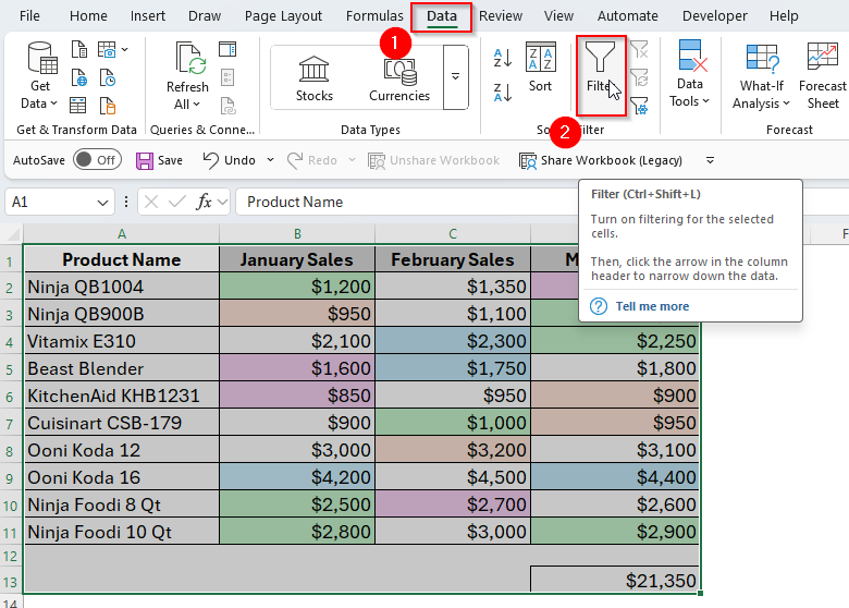
➤ Now select Data and then click on Filter as the image shows below.
➤ In the header cell, choose the Filter icon and then go to Filter by Color and select Green.
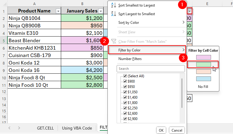
➤ Finally, the Green cells have been filtered and we’ve got the total sum in cell D13 .
Frequently Asked Questions
Why doesn’t SUMIF work with colors?
Because cell color is considered formatting, not a data value, and Excel formulas can’t directly read formatting without extra functions.
Is GET.CELL available in all Excel versions?
Yes, it is. But it’s an old macro function, so it only works through Named Ranges.
Concluding Words
So, this is all about Excel SUMIF cell color. The GET.CELL method is quick and doesn’t require macros, while VBA offers a more direct but slightly advanced solution. And if you just need a one-time total, filtering by color with SUBTOTAL might be the fastest.
With a bit of creativity, thus, we can make Excel’s SUMIF work like it was designed to handle colors from the start.