Normally, the SUMIFS function in Excel is used when we need to add up numbers based on multiple conditions. Most of the time, we use it for conditions like greater than, less than, or equal to. But what if you want to exclude certain text values while summing? That’s where we can use the not equal to text condition in Excel.
This is especially useful when your dataset contains different categories, product names, regions, or employee roles, and you want to sum values except for a particular text entry. For example, summing sales for all products except Apple Watch or anything like this.
Let’s go through it step by step.
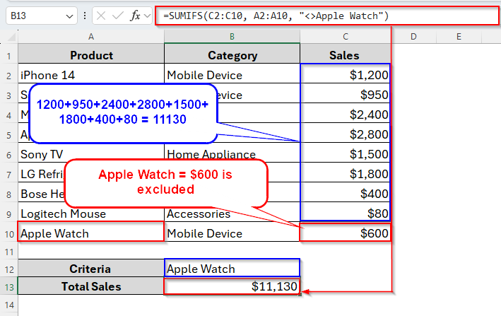
➤ Insert the following formula in cell B13:
=SUMIFS(C2:C10, A2:A10, “<>Apple Watch”)
➤ Press Enter and the total Sales values except Apple Watch will be calculated.
Fortunately, we can also apply this formula in multiple ways which is very handy and useful too. Let’s discuss in detail in the following parts of this article.
Overview of Excel SUMIFS Function
The SUMIFS function in Excel lets you sum numbers that meet more than one condition. Unlike SUMIF which allows only one condition, SUMIFS can handle multiple.
Syntax:
=SUMIFS(sum_range, criteria_range1, criteria1, [criteria_range2, criteria2], …)
➤ sum_range → The numbers you want to add.
➤ criteria_range1 → The cells Excel checks against the first condition.
➤ criteria1 → The actual condition.
➤ criteria_range2, criteria2 → Additional conditions (optional).
Example:
=SUMIFS(C2:C11, B2:B11, "<>HR")

Using SUMIFS with Not Equal to Text for Partial Matches
As we already know, the SUMIFS function allows us to exclude any word while summing up a specific range. That means it won’t count the cells referring to or related to that word. However, we can apply this formula for two different matches like partial matches and exact matches.
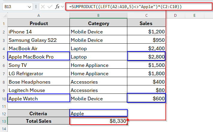
So, we usually use partial matches when we don’t want to exclude one exact word, but a group of words that share a pattern. For example, we’ve a product list of an electronics supplier company that includes the Product Names, their Category and Sales.
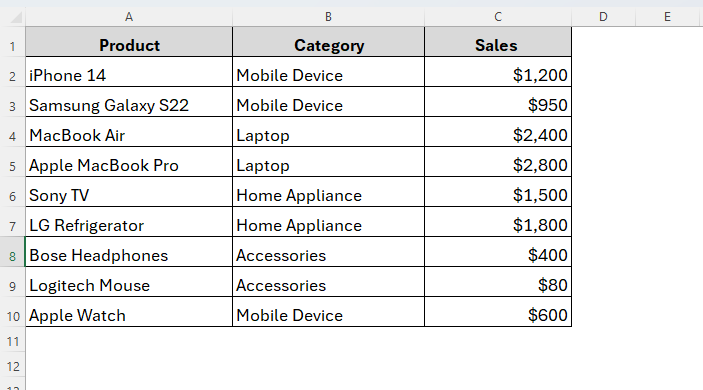
From the list, we want to exclude any word starting with Apple. To do so, we can apply the SUMIFS functions including wildcards with the not equal operator (<>). Here the asterisk (*), the most common wildcard in Excel, works like a placeholder for any characters after Apple. If you use it after Apple, Excel will skip all rows containing Apple at the beginning. In contrast, if you put it at the beginning of the word, it will skip all rows containing the word at the ending.
However, here we’re going to exclude cells beginning with the word Apple. And this is how it goes.
Steps:
➤ First, choose your criteria. Here our criteria is Apple.
➤ Next, type the following formula in cell B13:
=SUMIFS(C2:C10, A2:A10, "<>Apple*")
➤ Hit Enter and finally, the total count is here.
As we can see in the image above, it excluded two products Apple MacBook Pro and Apple Watch as they start with the word Apple. So, the Sales for these two products are also not counted.
Using SUMIFS with Not Equal to Text for Exact Matches
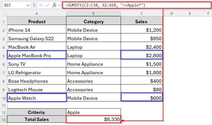
If we want to exclude any specific words like Apple Watch, then we have to follow this method. Unlike previous methods, it will only skip Apple Watch, not Apple MacBook Pro as we specified the word. Let’s see how it works.
Steps:
➤ Type the formula in cell B13 as follows:
=SUMIFS(C2:C10, A2:A10, "<>Apple Watch")
➤ Tap the Enter key. And as we can see in the following image, it adds up all values from the C2:C10 range, except for the Apple Watch ($600) from the A2:A10 range.
In this way, you can exclude any word from your dataset. Just replace Apple Watch with that word from your dataset.
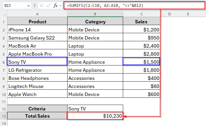
Applying SUMIFS for Not Equal to Text with Cell Reference
Instead of hardcoding the text directly in the formula, we can also make the criteria dynamic by using the cell reference. By doing so, you can change the word anytime without rearranging the formula and Excel will automatically generate the result.
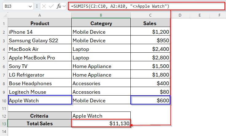
For example, we want to exclude the product LG Refrigerator while summing up. But we’ll do so by using cell reference. So, below are the steps to follow.
Steps:
➤ Enter the following formula in B13 cell:
=SUMIFS(C2:C10, A2:A10, "<>"&B12)
➤ Press Enter and here’s the result.
Here, the formula totals everything except the value from the cell B12, LG Refrigerator.
➤ Now if you change B12 to Sony TV, Excel will automatically update and exclude Sony TV instead.
Use SUMIFS Not Equal to Text with Multiple Criteria
Till now, we’ve just used a single criterion. But sometimes, we may need to apply more than one exclusion. For example, you might want to exclude both Mobile Device and Home Appliance from the sales total.
Fortunately, we can also do so by the SUMIFS function. This formula allows us to use multiple criteria at a time and make it more versatile from other functions like SUMIF.
Steps:
➤ Type the following formula in the cell B13:
=SUMIFS(C2:C10, B2:B10, "<>Mobile Device", B2:B10, "<>Home Appliance")
➤ Tap Enter and we’re ready to go.
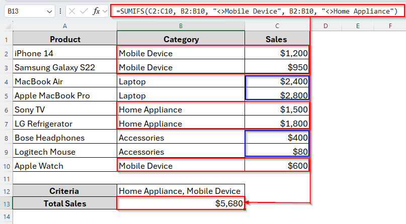
In the above image, you can see that we used multiple not equal criteria to get the total of the rest of the values.
Alternative to SUMIFS Function for Not Equal to Text Criteria
While SUMIFS works perfectly, it can get long and repetitive if you’re excluding multiple values. That’s when another Excel function, SUMPRODUCT, can be a cleaner and simpler alternative.
Use SUMPRODUCT for Not Equal to Text Condition
The SUMPRODUCT function can handle logical conditions in a more flexible way. The big advantage is that you don’t have to repeat the ranges multiple times like you do with SUMIFS.
For Partial Matches:
Steps:
➤ Type the following formula into cell B13 to get the result:
=SUMPRODUCT((LEFT(A2:A10,5)<>"Apple")*(C2:C10))
➤ Press Enter and the formula will sum the sales amount of the words with Apple only.
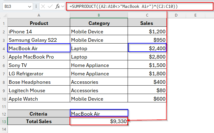
For Exact Matches:
Steps:
➤ Insert the following formula into cell B13:
=SUMPRODUCT((A2:A10<>"MacBook Air")*(C2:C10))
➤ Tap Enter after entering the formula. It will add the Sales values for products except MacBook Air.
Frequently Asked Questions
Can I exclude blank cells using SUMIFS?
Yes, you can. You just need to add another condition within the formula as follows:
=SUMIFS(C2:C11, A2:A10, “<>Apple”, A2:A10, “<>”)
That skips both Apple and extra spaces.
Can I Use Not Equal to Text for Case-sensitive Case?
By default, Excel text conditions are not case-sensitive. But there’s still a way. If you need case sensitivity, you’ll need an array formula or helper column.
What If My Text has Extra Spaces?
Extra spaces can cause errors because Excel treats “Apple ” (with a space) as different from “Apple.” To solve this, use the TRIM function or clean your data first.
Concluding Words
Using SUMIFS with not equal to text criteria gives you a quick and powerful way to filter out unwanted categories, products, or names while summing values in Excel. Whether you’re excluding one word, multiple entries, or partial matches, SUMIFS handles it smoothly.
And if you want even more control, switching to SUMPRODUCT can simplify things when conditions get more complex. So, next time you need totals excluding specific categories, remember these tricks. They’ll save you time, reduce manual filtering, and make your analysis more accurate.