How to Use SUMPRODUCT Function in Excel with Multiple Criteria

When it comes to sum a range of data while handling multiple conditions in Excel, we often start to fumble. Most of the time, we jump to the SUMIFS formula without thinking twice. But what if you need more flexibility and control over your data? In cases where you need to combine only conditions from the others, work with numeric thresholds, or even find weighted sums – SUMPRODUCT is your savior. It works beyond typical SUMIF and helps you work with multiple criteria across texts, numbers, arrays, or whatever you ask.

When adding cell values based on specific criteria, SUMPRODUCT is the best fit. It allows both conditions to be met before applying the summation. Do not bind your dataset to a particular structure. With SUMPRODUCT, you can evaluate each row individually, multiply those results, and finally add the values together to give the result.

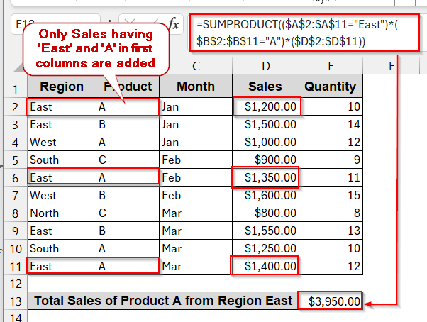
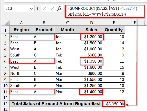
To illustrate this method, we will find out the total sales from the Region East and Product A. This means our criteria will be ‘East’ from column A (Region) and ‘A’ from column B (Product).

Steps:

➤ Look for the columns and cells that contain the required criteria.
➤ Select a cell to write the formula. Represent it with an appropriate header.
➤ Write the SUMPRODUCT formula –

Here, $A$2:$A$11=”East”  ensures the cells of A2 to A11 have ‘East’, while $B$2:$B$11=”A” ensures the B cells of this range contain ‘A’. The total sum is applied to columns D2 to D11.

➤ Press Enter to get the results.

➤ Change the criteria to see if the result changes or not.

Two conditions are just best suited for examples. Your main dataset often requires working with three or multiple criteria to satisfy before summing them up. However, like your data, the SUMPRODUCT also has no limits. You can stack your conditions one after another in the formula, and everything will work perfectly fine.

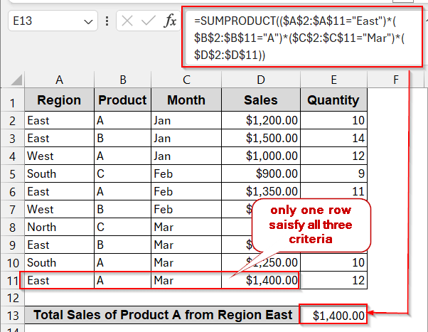
This time, we will only find the total sales of Product A from Region East in March. Therefore, we now have three criteria: ‘East’, ‘A’, and ‘Mar’.

Steps:

➤ List the conditions and check all the columns that are used.
➤ Select the cell to write your result.
➤ Give it a proper header to present itself.
➤ Place the following formula in the selected cell –

$A$2:$A$11=”East”, $B$2:$B$11=”A”, $C$2:$C$11=”Mar” are the conditions that are multiplied together. This ensures that only the rows with all three are filtered out from column D.

➤ Press Enter to see the results.

So far, we have discussed situations having textual criteria, more from the data value itself. But the real worksheet problems may lie deeper down. Oftentimes, you need to compare numeric values as a criterion to get the sum of the results. This is where SUMPRODUCT is uniquely used. Unlike SUMIFS, it can work with numeric operators like  ‘>’, ‘<’, ‘>= ’, and ‘<=’.

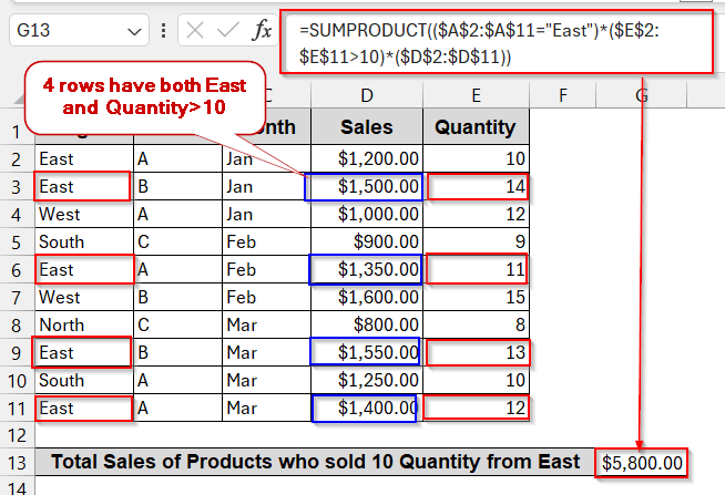
As a heads up for this method, we will try to find out the total sales from Region East that have sold more than 10 quantity. So, our criteria will be region ‘East’ and Quantity>10.

Steps:

➤ Identify the conditions and columns associated with this. (e.g, column A (Region) and D (Quantity).
➤ Select an output cell to write the results.
➤ Give it a proper header.
➤ Write the formula of SUMPRODUCT

First condition – $A$2:$A$11=”East” (column A needs to have ‘East’)
Second condition – $E$2:$E$11>10 (column E needs to have a value greater than 10)

➤ Press Enter to get the result in the cell.

➤ Try changing the criteria and see how your result changes dynamically.

SUMPRODUCT logic can be classified into two categories: AND and OR. The previous examples are all AND logic. That means all the conditions must be satisfied. When and only when all are satisfied, the row is filtered out, and the result is summed. On the other hand, the OR logic works differently. When SUMPRODUCT is used with OR logic, it filters out all the rows that fulfill at least one criterion (even if not all). The AND logic is represented by the multiplication sign (*) while the OR is denoted with the addition sign (+).

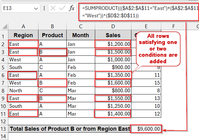
In this scenario, we will find the total sales if the product is B or from the region East. That suggests we have two conditions, one is Region ‘East’ and the second is Product ‘B’. Any one of them must be true for the SUMPRODUCT to work.

Steps:

➤ Define the conditions and locate the columns that are included. Here, column A and B are included for ‘East’ and ‘B’ respectively.
➤ Find a cell to display your output. If needed, give a proper header.
➤ In the selected cell, write down the SUMPRODUCT formula –

➤ Press Enter to get the result.

➤ Change the criteria to see how the result gets changed.

In real-world situations, problems are rarely simple. They often include mixed forms of criteria, ranging from text, numeric, and AND/OR logics. As hard as it sounds, the SUMPRODUCT has an easy solution.

Here, we will find the total sales from the Region East or West of product A that have sold more than 12 units. To put it simply, we have three conditions here – the Region has to be either ‘East’ or ‘West’, the Product must be ‘A’, and the Quantity must be greater than 12.

Steps:

➤ Break down the conditions and identify the columns and cells involved.
➤ Select a cell to display the output.
➤ Give it a proper header.
➤ Write the OR logic for the Region part –

–(($A$2:$A$11=”East”)+($A$2:$A$11=”West”)>0),

Here, the formula is wrapped with — and >0 to keep the result in binary (1 when at least one is TRUE, otherwise 0 for FALSE).

➤ Write the Product criteria, combining them with AND logic.

*($B$2:$B$11=”A”)

➤ For the Quantity condition, use this –

*($E$2:$E$11>12)

➤ Combine all the conditions inside the SUMPRODUCT.

➤ Press Enter to get the result in the cell.

SUMPRODUCT is the easiest and most straightforward solution for complex problems. But that does not mean you can’t make it more friendly and dynamic with some automation. Combining these SUMPRODUCT formulas with the VBA Macros to work it like a simplified function.

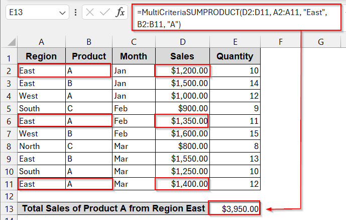
With VBA Macros, we will make a custom function that will calculate the total sales of Product A from Region East.

Steps:

➤ Open the dataset and go to the Developer tab. Select Visual Basic from there.

➤ In the launch VBA editor window, go to the Insert option and select Module.

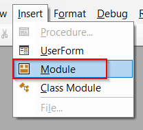
➤ In the blank space, paste the following VBA code snippet.

Function MultiCriteriaSUMPRODUCT(SumRange As Range, ParamArray Criteria() As Variant) As Double
    Dim i As Long, j As Long
    Dim Result As Double
    Dim Include As Boolean
    For i = 1 To SumRange.Rows.Count
        Include = True
        For j = LBound(Criteria) To UBound(Criteria) Step 2
            If Criteria(j).Cells(i, 1).Value <> Criteria(j + 1) Then
                Include = False
                Exit For
            End If
        Next j
        If Include Then
            Result = Result + SumRange.Cells(i, 1).Value
        End If
    Next i
    MultiCriteriaSUMPRODUCT = Result
End Function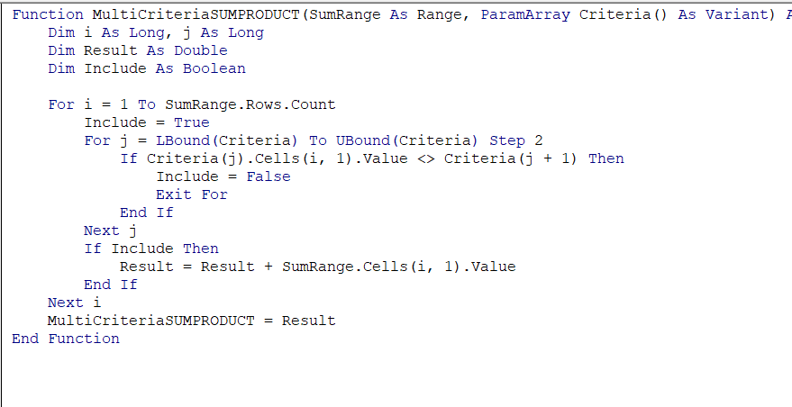

➤ Click  Ctrl  +  S  to save the VBA snippet. After saving, close the editor.
➤ Select a cell to write the newly customized function. Give it a proper header.
➤ Write the formula below –

Here, MultiCriteriaSUMPRODUCT is the name of the VBA-created function. The first parameter is the resultant column range; the rest are column ranges followed by the criteria.

➤ Press Enter to get the result.

Frequently Asked Questions (FAQs)

Can SUMPRODUCT handle text, numbers, and dates together?

SUMPRODUCT can handle both texts, numbers, and dates all at once. You can combine all these criteria with AND or OR logic and mix different data types. No need to use a separate function.

Why is my SUMPRODUCT returning #VALUE?

SUMPRODUCT might throw a #VALUE error due to an uneven column range. For example, if the criteria column range is from A2 to A11, the sum range also must be from D2 to D11. If they are not the same, the result displays #VALUE.

Is SUMPRODUCT slower than SUMIFS on large datasets?

SUMPRODUCT is slower than SUMIFS. As SUMPRODUCT evaluates the result row by row and one criterion at a time, it might feel slower in large datasets.

Is SUMPRODUCT better than SUMIFS?

SUMPRODUCT is the better alternative to SUMIFS. SUMPRODUCT can combine multiple criteria of multiple types. It includes AND/OR logic and enables users to include numeric conditions too, which is absent in SUMIFS.

Can I replace all SUMIFS with SUMPRODUCT?

Technically, you can replace SUMIFS with SUMPRODUCT. However, it might lag the performance and even affect the result due to the syntax and the AND/OR logic.

Concluding Words

Mastering the SUMPRODUCT formula gives you more flexibility than relying on typical formulas. From handling multiple criteria ranging from texts and numerics, you now know how to handle different logical operations like AND and OR. As you learn them by heart, you can level up your worksheet management with automated VBA methods. By blending these methods and finding the best fit, you can work with any dataset size with accuracy, speed, and confidence.