The VLOOKUP function is one of Excel’s most common tools for finding data, but sometimes a single lookup isn’t enough. When your information is split across multiple tables, you may need to run one lookup inside another. This is called nested VLOOKUP.
With nested VLOOKUP, you can first retrieve an intermediate value, such as a category or code, and then use that result to perform another lookup that returns the final answer. It’s a practical way to connect related tables and automate multi-step searches.
In this guide, we’ll show you how to apply nested VLOOKUP step by step.
Here’s how to use nested VLOOKUP in Excel:
➤ Open your dataset in Excel.
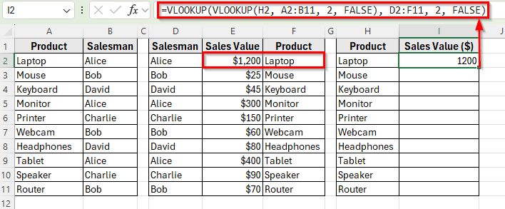
➤ Click on cell I2 which is next to the first product in the results section.
➤ Enter the following formula:
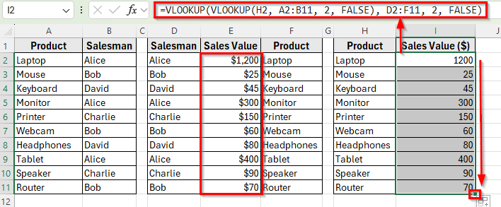
=VLOOKUP(VLOOKUP(H2, A2:B11, 2, FALSE), D2:F11, 2, FALSE)
➤ Press Enter. Excel will display the Sales Value for the first product. For example, 1200 for Laptop.
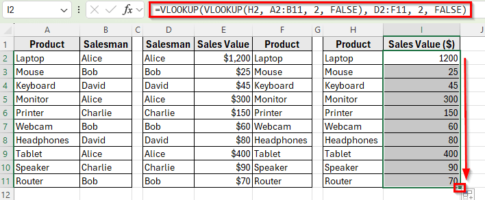
➤ Drag the fill handle down to apply the formula to the rest of the rows in Column I. Each product will now show its correct Sales Value.
What Is Nested VLOOKUP in Excel?
A nested VLOOKUP means placing one VLOOKUP formula inside another. The first VLOOKUP finds an intermediate value, and the second VLOOKUP uses that value to return the final result.
This method is useful when your data is stored in different tables and you need to connect them. For example, you may first look up a Salesman to get their Product, and then use that Product to find the related Sales Value.
Generic Syntax:
=VLOOKUP(VLOOKUP(lookup_value, table_array1, col_index_num1, FALSE), table_array2, col_index_num2, FALSE)
Nested VLOOKUP to Return Sales Value for Each Product in Excel
In the following dataset, we have a product sales log that links items with the salesmen who sold them. Column A contains the Products, and Column B shows the Salesmen responsible for each sale.
To the right, another table provides more details about each salesman. Column D lists the Salesman Names, Column E shows their Sales Values, and Column F contains the Products they sold.
Finally, we’ve prepared a results section with Products in Column H. Our goal is to use nested VLOOKUP to return the correct Sales Value for each product and display it in Column I.
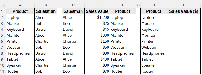
We’ll use this dataset to demonstrate step by step how nested VLOOKUP works in Excel.
In this method, we’ll use a nested VLOOKUP formula to pull the Sales Value for each product. The formula will first look up the Salesman for a product, and then use that Salesman to return the matching Sales Value from the second table.
Here’s how to apply this method:
➤ Open your dataset in Excel.
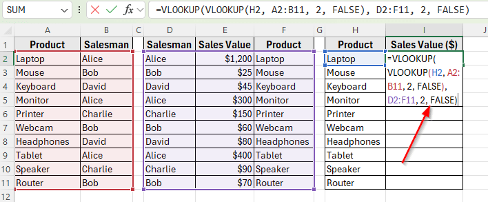
➤ Click on cell I2 which is next to the first product in the results section.
➤ Enter the following formula:
=VLOOKUP(VLOOKUP(H2, A2:B11, 2, FALSE), D2:F11, 2, FALSE)
➤ Press Enter. Excel will display the Sales Value for the first product. For example, 1200 for Laptop.
➤ Drag the fill handle down to apply the formula to the rest of the rows in Column I. Each product will now show its correct Sales Value.
Nested VLOOKUP to Return Product by Salesman
In this method, we’ll use nested VLOOKUP to find which Product is linked to a given Salesman. The formula will first locate the Salesman in the main table and then use that result to return the corresponding Product in the result table.
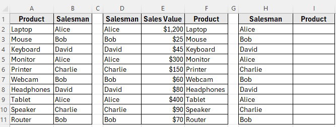
In our dataset, we’ve made some changes. Now column H is listed with Salesman Names and column I is labeled Product, which is currently empty. We’ll apply a nested VLOOKUP formula in column I to return the correct Product for each Salesman.
Here’s how to apply this method:
➤ Open your dataset in Excel.
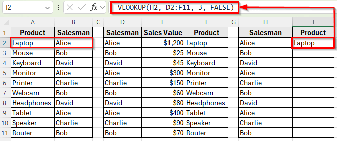
➤ Click on cell I2 which is next to the first product in the results section.
➤ Enter the following formula:
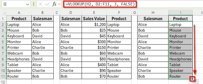
=VLOOKUP(H2, D2:F11, 3, FALSE)
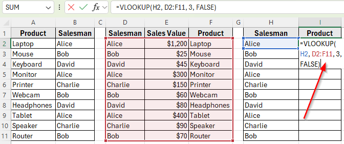
➤ Press Enter. Excel will display the first Product sold by that Salesman. For example, Laptop for Alice.
➤ Drag the fill handle down to apply the formula for the rest of the rows. Each row will now show the corresponding Product for the Salesman listed in column I.
Frequently Asked Questions
What is a nested VLOOKUP in Excel?
A nested VLOOKUP is when you use one VLOOKUP formula inside another. The first VLOOKUP helps find the lookup value, and the second VLOOKUP retrieves the actual result you want. This is useful when the value you’re searching for is linked across multiple tables.
Why should I use nested VLOOKUP instead of a normal VLOOKUP?
A normal VLOOKUP works when all the information you need is in one table. Nested VLOOKUP is helpful when your data is split across two or more tables, and you need to connect them to pull the final result.
What happens if the nested VLOOKUP does not find a match?
If no match is found, Excel will return a #N/A error. To handle this, you can wrap the formula with the IFERROR function, for example:
=IFERROR(VLOOKUP(VLOOKUP(H2,$C$2:$D$11,2,FALSE),$A$2:$B$11,1,FALSE),"Not Found")
Wrapping Up
Nested VLOOKUP is a simple way to connect data across multiple tables in Excel. By using one lookup inside another, you can return the right result even when the information is split into different lists.
It’s especially helpful when working with datasets that link salesmen, products, and values. With just one formula, you can bring everything together and make your data easier to understand.