The VLOOKUP function in excel is designed to return the first match it finds. But what if your dataset contains duplicate entries and you want to pull the second match instead? While VLOOKUP doesn’t support this directly, we can use a helper column to vlookup the second occurrence of a matching value in a dataset.
This method involves tagging repeated values with a unique counter, so we can use VLOOKUP on a more controlled and structured lookup key. It’s especially useful when dealing with names, product IDs, or transaction logs where duplicates are common.
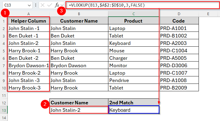
➤ To begin with, create a helper column on the left of the first column.
➤ Then insert the customer name for the second match in cell B13.
➤ Now enter the following formula in cell C13.
=VLOOKUP(B13,$A$2:$D$10,3,FALSE)
➤ Hit the Enter key and here we go.
Now, let’s walk through an example to understand how this method works in a real dataset. We’ll also explore some alternatives, so you can simply apply the best method for your task. Let’s dive in.
Vlookup Second Match Using a Helper Column
Usually, the VLOOKUP function in Excel only returns the first match depending on a single lookup value we specify. To tackle this feature, as we’ve already mentioned earlier, we can simply add a helper column and link the values from two lookup columns (here, Customer and Product).
Today, we have a dataset of customers and the products they purchased. But some customers also appear more than once. Let’s assume, we want to find out the second product purchased by a customer named John Stalin.
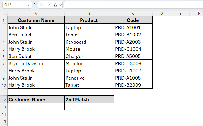
Since VLOOKUP normally only gives the first result, we’ll solve this using a helper column. Let’s see how it goes.
Steps:
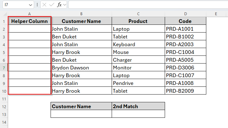
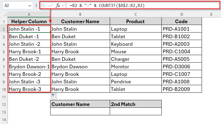
➤ Insert a new column just to the left of column A. Now column A will turn into a helper column and the previous column A is converted to column B as we can see in the image below.
➤ Now type the following formula in cell A2:
=B2 & "-" & COUNTIF($B$2:B2,B2)
➤ Press Enter and drag the AutoFill Handle down to cell A10. After this step, the helper column will be as follows.
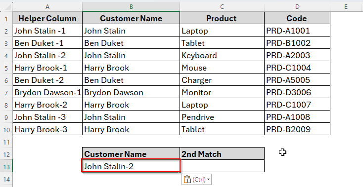
➤ Now we’ll enter a lookup key in cell B13. The lookup key is the unique key that refers to John Stalin’s second entry. So, in cell B13, type John Stalin-2.
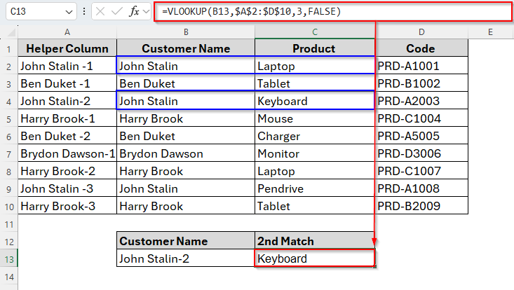
➤ Finally, insert the following formula in cell C13.
=VLOOKUP(B13,$A$2:$D$10,3,FALSE)
➤ Press Enter and the result is Keyboard which is the second product purchased by John Stalin.
Vlookup Second Match without Using a Helper Column
If you don’t want to create the helper column to vlookup the second match in your dataset, well Excel also offers some alternatives you can choose from. These alternatives don’t modify your data using a helper column. Therefore, you use a direct formula and get the results.
Let’s find out two most significant and useful formulas while looking up the second match in excel. One is combining the INDEX, SMALL and IF functions and another is using the FILTER and INDEX functions together.
Using INDEX, SMALL, and IF Functions
The most useful part of this method is that the entire logic is in a single formula. Unlike the VLOOKUP function, we can easily look beyond the first match and get the second, third or even Nth match with this method.
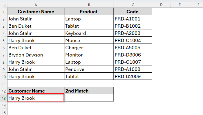
It also works great even if you have a large list of repeated values. For example, now will find the second product purchased by the customer named Harry Brook from our today’s dataset. Let’s find it out.
Steps:
➤ Enter the name Harry Brook in cell A13.
➤ Now in the cell B13, insert the formula as follows:
=INDEX(B2:B10, SMALL(IF(A2:A10=A13, ROW(A2:A10)-ROW(A2)+1), 2))
➤ Press Enter and the second product purchased by Harry Brook, Laptop will appear in the same cell.
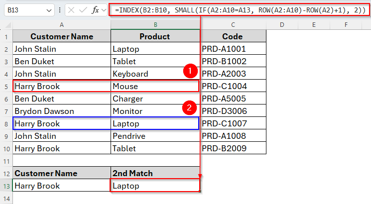
Here, the IF function detects all rows where the name Harry Brook is and gives the row numbers in a list. Then the SMALL function picks the second smallest row number from that list, meaning the second time Harry Brook appears. Finally, INDEX chooses and returns the value (Product) from column B based on that list.
Using the FILTER and INDEX Functions
This is another simple and modern method available in Excel 365 and Excel 2021. These are usually some powerful dynamic array functions that can easily return not only the first match but also the second, thor or Nth matches.
Moreover, the method is short, simple and super easy to apply. It doesn’t require any helper columns or array formula. You can easily change the match number just like 2 to 3, 4 etc. and you’ll get the required match.
Now, we’ll again find the second occurrence of the customer named John Stalin using the FILTER and INDEX functions. Below are the steps to follow:
Steps:
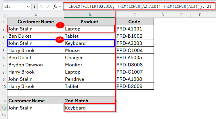
➤ Type the name John Stalin in cell A13.
➤ Then insert the following formula in cell B13.
=INDEX(FILTER(B2:B10, TRIM(LOWER(A2:A10))=TRIM(LOWER(A13))), 2)
➤ Tap Enter and the second match for John Stalin Keyboard will appear as we can see in the following image.
Frequently Asked Questions
What happens if there’s no second match?
If no second match exists, the formula will return an error like #NUM! or #N/A. You can handle this with IFERROR.
Can I get the third, fourth, or nth match in Excel the same way?
Yes. Just change the number inside the formula. For example, replace 2 with 3 for the third match, 4 for the fourth, and so on.
Which is better for second match lookup — array formulas or helper columns?
It actually depends. Array formulas (INDEX + SMALL) are flexible but can be complex while Helper columns make formulas simpler and easier to maintain.
Concluding Words
Finding the second match in Excel may seem tricky at first since the standard VLOOKUP function only fetches the first result. But with a little creativity, it becomes quite easy and manageable. Whether you choose to use a helper column, the INDEX-SMALL-IF combination, or the more modern FILTER and INDEX functions, each method offers a smart way to work around Excel’s limitations when handling duplicates.
The helper column is best for structured datasets where you want to visually track each match. On the other hand, the formula-based approaches are more dynamic, flexible, and ideal when you want to keep your data clean and untouched.
Ultimately, your choice will depend on the Excel version you’re using, the size of your dataset, and how often you need to retrieve repeated matches. Try them out and use whichever method best fits your workflow.