Pivot Tables are used for summarizing and analyzing vast amounts of data in Excel. However, the summarized results often need to be presented on a separate sheet for further analysis. Linking a Pivot Table data to another sheet ensures that the reports are dynamic and automatically update whenever the underlying Pivot Table changes. In this article, we will guide you through three powerful methods for linking Pivot Table data, ranging from a simple direct reference to a dynamic solution.
To link Pivot Table data to another sheet in Excel, here is one simple solution by using the cell reference.
➤ To link a single cell, choose a cell in a separate sheet and type equal (=).
➤ Go to the Pivot Table sheet and click the cell that you need to link.
➤ Press ENTER, and you will get the Pivot Table data in a different sheet.
Using Direct Cell References to Link Single Cell
This is the simplest way to connect a reporting cell to a Pivot Table. While quick to set up, it creates a static link that is highly vulnerable to changes in the Pivot Table’s layout. You can use this method only when the Pivot Table structure will not change.
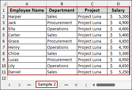
Imagine we have a dataset named “Sample 1” containing employee records with names, departments, projects, and salaries. First, we will create a Pivot Table based on this data and then link the Pivot Table data to another sheet.
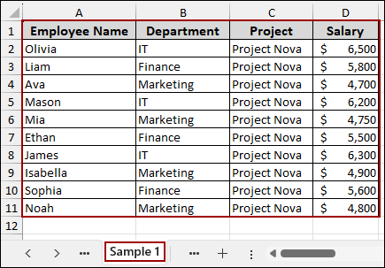
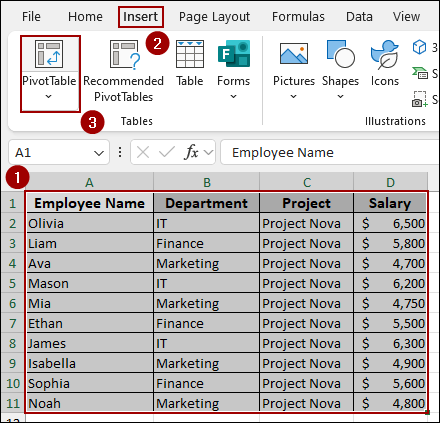
➤ Select the entire dataset in the “Sample 1” sheet.
➤ Go to the Insert tab and click PivotTable.
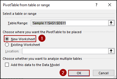
➤ In the dialog box, ensure New Worksheet is selected and click OK.
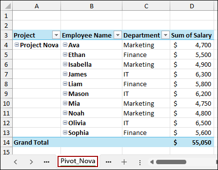
In the new sheet, we will name the sheet “Pivot_Nova”. After dragging Project, Employee Name, and Department to the Rows area, and Salary to the Values area, our Pivot Table will look like the image below.
Now, we will link this Grand Total to a new sheet named “Single Cell” using a direct cell reference.
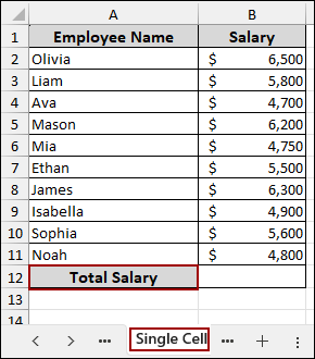
➤ In the “Single Cell” sheet, select the cell where you want the total to appear (B12) and type an equal sign (=).
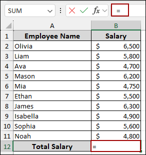
➤ Navigate to the “Pivot_Nova” sheet and click the cell containing the Grand Total ($55,050 in D14).
➤ Press ENTER.
The result $55,050 is pulled from the Pivot Table. This way, you can easily link Pivot Table data to another sheet in Excel.

Applying GETPIVOTDATA Function to Link Specific Data from Pivot Table
The GETPIVOTDATA function in Excel is designed to link data from the Pivot Table. It retrieves data based on field names and items, making the link stable. This method is dynamic as it won’t break when the Pivot Table is updated.
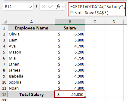
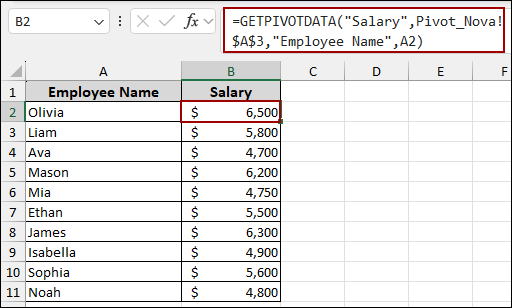
Suppose we have only the employee name in a separate sheet. Now, we will extract all employees’ salaries from the Pivot Table using a simple formula.
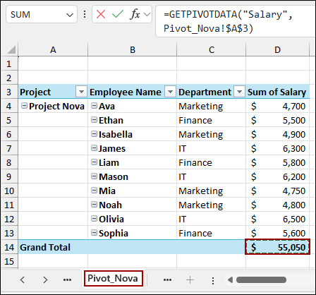
➤ Select cell B2, enter the formula below, and drag the Fill Handle down.
=GETPIVOTDATA("Salary",Pivot_Nova!$A$3,"Employee Name",A2)
In this formula, we have added a field/item pair, “Employee Name” is the field, and A2 is the cell reference containing the item (Olivia). This formula dynamically pulls Olivia’s salary of $6,500. By dragging this formula down, the cell reference will change, linking the salary for every employee listed in column A.
Combining INDIRECT and GETPIVOTDATA Functions to Link Multiple Pivot Tables
For advanced scenarios, you can use the method below to dynamically pull data from multiple Pivot Tables on different sheets. By using the combination of GETPIVOTDATA and INDIRECT functions, you can build a flexible reference that changes the source Pivot Table based on a selection.
We will introduce a second dataset named “Sample 2”, detailing employees working on a different project named Luna.
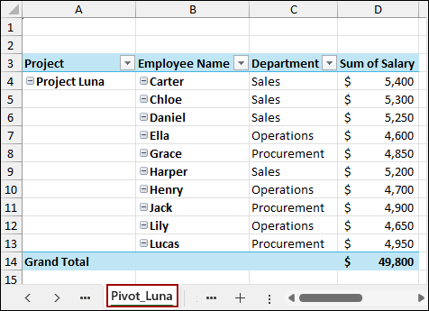
➤ Create a second Pivot Table from this data, structuring it identically to the first.
➤ Name this new sheet “Pivot_Luna”.
In a new sheet named “Multiple Pivot Table”, we will set up a dropdown list to switch between the two projects.
➤ Select cell A2.
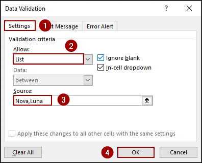
➤ Go to the Data tab, click on Data Tools, and select Data Validation.
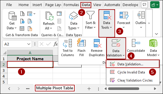
➤ In the Data Validation dialog box, set the Allow criteria to List.
➤ In the Source field, type the short names of the projects/sheets: Nova,Luna.
➤ Click OK.
As a result, cell A2 now has a dropdown menu allowing you to select Nova or Luna.
➤ Click the drop-down arrow and choose Nova.

Now, we use the combined formula to link the salary dynamically based on the project selected in cell A2.
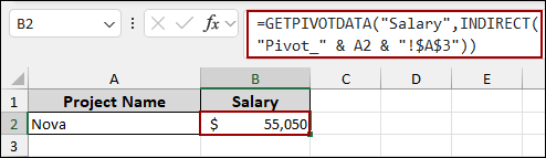
➤ In cell B2, enter the following formula and press ENTER.
=GETPIVOTDATA("Salary",INDIRECT("Pivot_" & A2 & "!$A$3"))
With “Nova” selected in A2, the formula returns the total of $55,050.
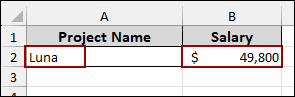
If you change the selection to “Luna”, the formula automatically updates the Pivot Table reference to Pivot_Luna and returns $49,800.
Frequently Asked Questions
Why do I get a #REF! error when using GETPIVOTDATA?
The #REF! error typically occurs if the Pivot Table reference is invalid or if the field/item combination you specified does not exist in the Pivot Table.
How do I stop Excel from automatically generating the GETPIVOTDATA function when I click on a Pivot Table cell?
Excel is designed to automatically insert the function when you type equal (=) and click a value inside a Pivot Table. To disable this, go to the PivotTable Analyze tab. In the PivotTable group, click the Options drop-down arrow and uncheck the option Generate GetPivotData.
Can I reference a calculated field or item in the Pivot Table?
Yes. The GETPIVOTDATA function can extract data generated by Excel’s Calculated Fields or Calculated Items. You need to use the name of the calculated field as the data_field argument.
Concluding Words
Above, we have explored three key methods for linking Pivot Table data to other sheets, ranging from the simple direct reference to the combination of GETPIVOTDATA and INDIRECT functions. While the direct link is fast, the true utility lies in the dynamic capabilities offered by the GETPIVOTDATA function. Following these methods, you can easily link Pivot Table data to another sheet based on your preference. If you have any questions, please don’t hesitate to share them in the comments section below.