While working with pivot tables, you might have encountered the error that says “The Pivot Table Field Name is Not Valid”.There could be a number of reasons that can lead to this error. In most cases, this error is caused by some issues in the source data. In this article, we will show you all possible reasons for this error and how to fix the issue in no time. Soon, you will be able to get back to analyzing your data like before.
➤ In the source data, find the column that does not have a header.
➤ Put a header on that column, and then try to create the pivot table.
While that fix should work for most cases, it might not fix the issues for your worksheet. In this article, we will have more causes and solutions to the problem, so that you can try them all and fix your pivot table. Therefore, read the whole tutorial and make sure to follow the steps mentioned in each method carefully.
Check for Missing Header
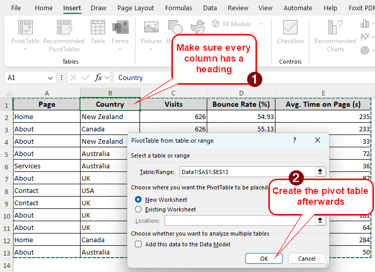
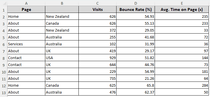
To demonstrate this method, we have a dataset of website traffic. There are page names, visits, the bounce rates, the average time people spent on pages, and the countries they visited the pages from. Let’s try to pivot this table.
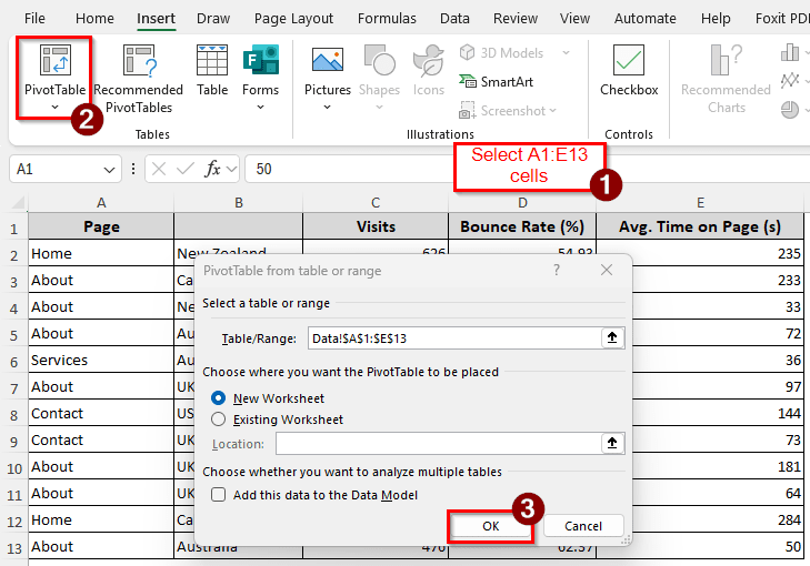
➤ Select A1:E13 cells, and go to the Insert tab from the ribbon at the top of Excel. From the Tables section in that tab, click PivotTable.
➤ Press OK to try to create the table. However, it should not work and show an error.
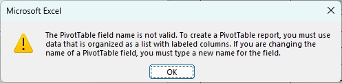
➤ That happened because the B1 cell is blank. Excel counts the top row as the heading, and if there’s no heading, there’s no pivot table. Let’s write “Country” in there.
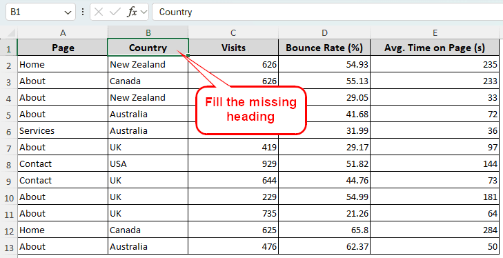
➤ Now, if we try to create the pivot table again, it works perfectly.
Unhide Columns to Check for Issues
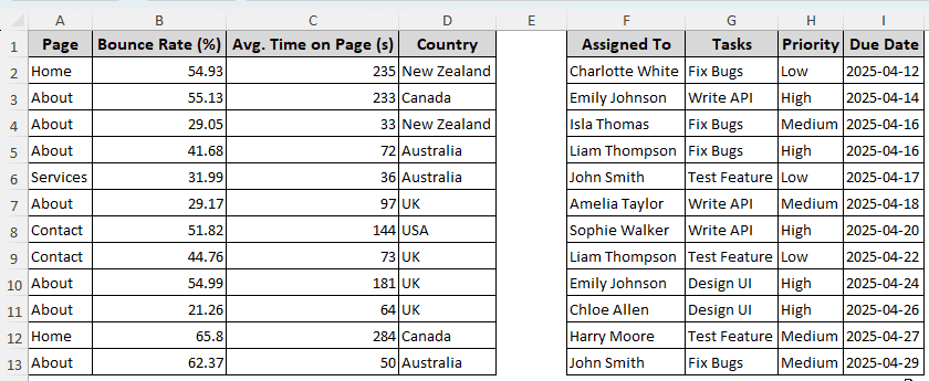
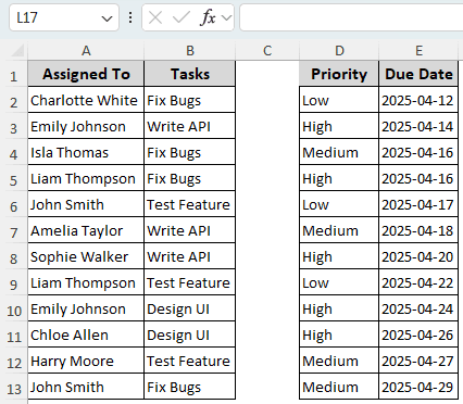
Let’s have a look at another table. This one is about project tasks. There are task names, who they are assigned to, the priorities of the tasks, and the due dates. Apparently, every column has headings, so there should be no issues.
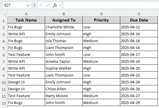
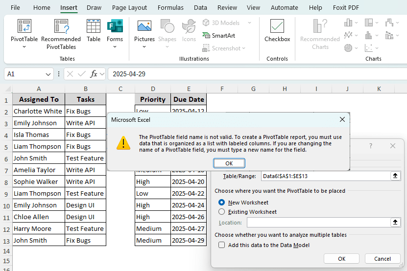
➤ When we try to create a pivot table with this dataset, we face an issue again.
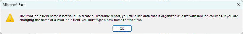
➤ The issue here is that there is a hidden column with missing headers. There is no C column in this dataset.
➤ To solve that, select both B and D columns, right-click, and hit Unhide.
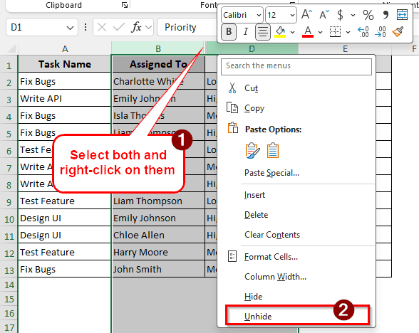
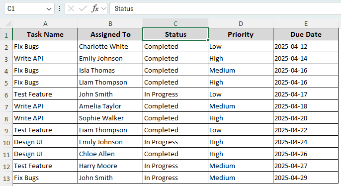
➤ Now we can see that the hidden column had no heading. We can give the C column a heading to fix the issue.
➤ The pivot table creation becomes successful now.
Unmerge Headings to Fix the Error
For this method, we have the same dataset from the previous one, but a bit modified to help demonstrate the issue. The tasks and the statuses are in two separate columns, but have the same heading. As a result, the pivot table cannot be created. Follow the steps to learn how to fix that:
➤ Select B1 cell, and head to the Home tab. From there, go to the Alignment section. Open the dropdown of Merge & Center, and select Unmerge cells.
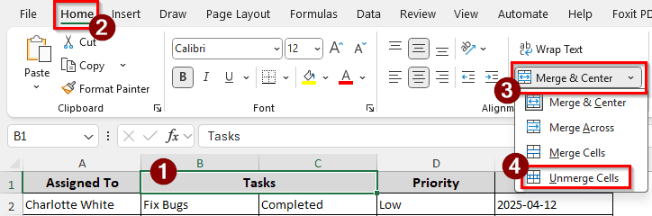
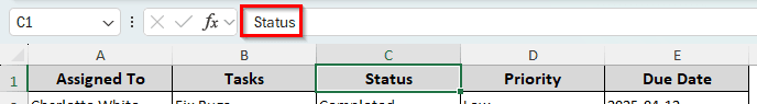
➤ Now the cells are unmerged, but we still have to put a heading for C1. Write “Status” in that cell and create the pivot table.
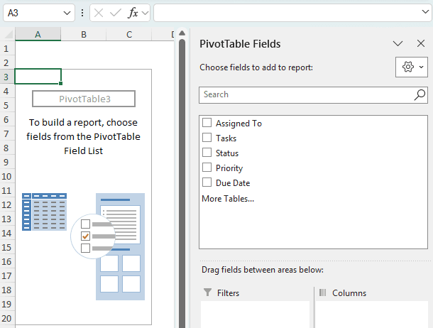
➤ Now the pivot table can be created and customized as required.
Select the Range Properly
Sometimes, while creating pivot tables, we don’t select the table properly. Instead, we press Ctrl + A and try to make the pivot table with the whole sheet. This small mistake makes it impossible to create the pivot table. Take a look at the following case. We have two tables in a single sheet for this example:
➤ If we try to create a pivot table by pressing Ctrl + A and going to Insert > PivotTable, it won’t work and throw up an error.
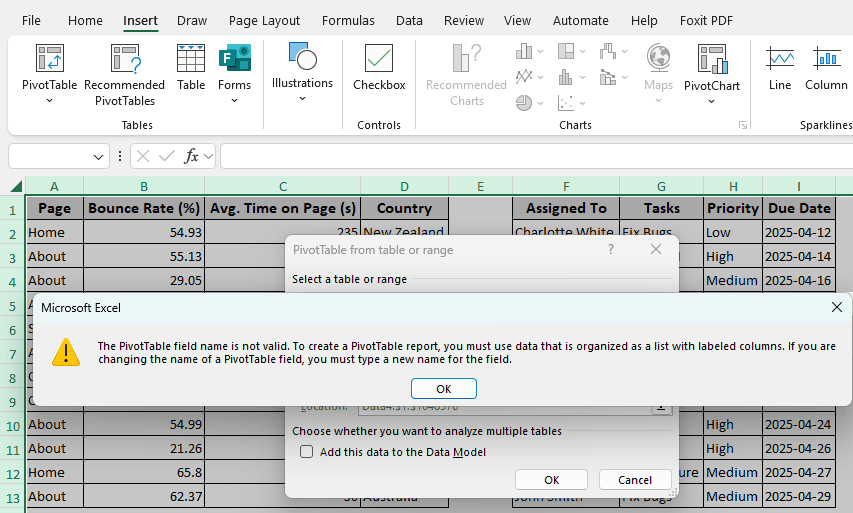
➤ The issue is, Excel considers the whole top row as the heading. There are two tables here, and there is a gap in the E column. Excel got confused by the gap and refused to create the pivot table.
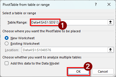
➤ To fix the issue, select the range properly. Either select A13:D13 or F13:I13 to create a proper pivot table.
➤ Here is the resulting pivot table.
Look for the Missing Dataset
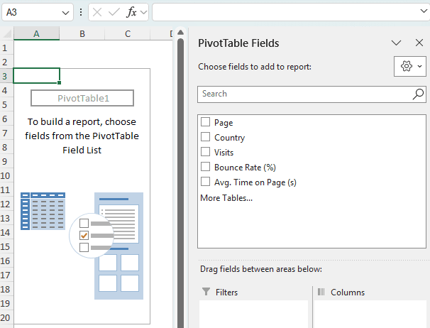
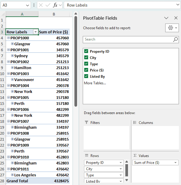
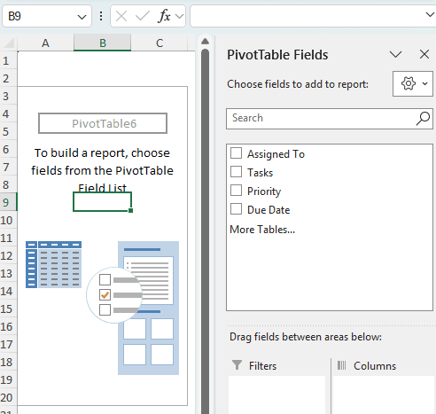
Here, we have a pivot table with some property valuations. The PivotTable Fields section makes it clear that there are five fields in the table. There are property IDs, the cities where the properties are, the types of those properties, the prices, and who listed them.
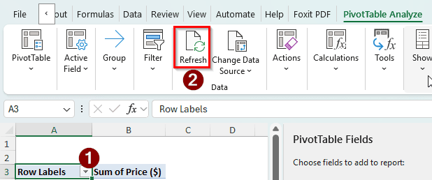
➤ There are no issues if we look at the pivot table like this. But we might need to refresh the dataset at some point.
➤ Click on any cell of the pivot table (we are clicking on A3 here), and go to the PivotTable Analyze tab.
➤ Click Refresh from the Data section.
➤ Now the pivot table shows the well-known error.
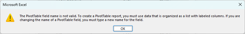
➤ There is no fix after you see this message. To make sure that this error does not happen, do not delete the source dataset after creating the pivot table. Once you delete the dataset and have no means of recovering, this error will keep showing up.
Fix Missing Columns
The dataset we have currently belongs to the same table. But there is a column gap between them for some reason, and the pivot table cannot be created because of that. Here is how we can fix that:
➤ If we try to create a pivot table using the A1:E13 cells in the current state, we will get an error.
➤ To fix the issue, select D1:E13 and press Ctrl + X .
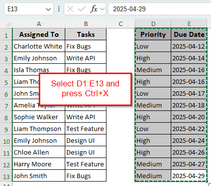
➤ Go to the C1 cell, and press Enter.
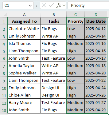
➤ Now try to create the pivot table with the range of A1:D13. It should work properly.
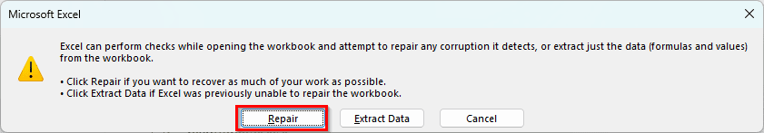
Repair the Excel File
When everything else fails, you can try fixing the Excel file to fix the issue.
➤ Open Microsoft Excel.
➤ Go to Open > Browse. Now, find the Excel file with the issue, and select it. From the dropdown menu of the Open button, select Open and Repair.
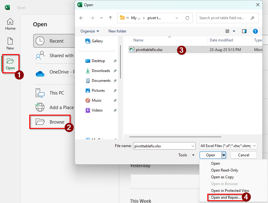
➤ Press Repair to repair the Excel file.
Frequently Asked Questions
Why is my data not valid for a pivot table?
Make sure you don’t have any special characters in the filename of the Excel sheet. There are some rules in the naming scheme of files and windows. Always adhere to those rules to get rid of these errors.
How to fix the pivot table field name already exists?
Go to your dataset and check the names of the columns. If multiple columns have the same name, that will cause this issue. Rename those columns and make sure every column has a separate name.
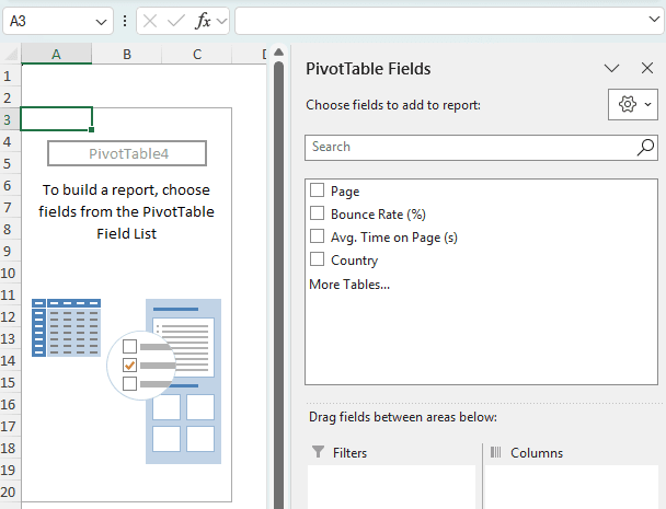
How to use PivotTable fields?
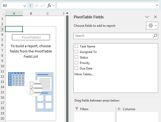
The PivotTable Fields section contains the fields from the source data. You can drag and drop the fields to the Rows, Columns, Values, and Fields sections to manipulate the pivot table. You can also check the boxes of the fields to make a pivot table automatically.
Why is my PivotTable saying data source not valid?
Either you have changed the data source massively, or you have deleted the dataset by accident. The pivot table does not have a source right now to refresh the data from, and that is causing the error.
How do you reset PivotTable options?
The easiest way to do this is to create the pivot table entirely. If you got the pivot table from a colleague and have no way of knowing what settings they have changed, it is better to just create a new pivot table with the existing data source.
Wrapping Up
In this article, we have learned how to fix the “field name is not valid” error of a pivot table. We hope that you were able to resolve the issues you were having with your pivot table after reading this article. If you are still facing errors, leave your issue in detail below so that we can take a look. Until next time, stay tuned.