If you have closed the “PivotTable Fields” menu by accident, you are probably having issues managing your pivot table. The “PivotTable Fields” menu allows us to dynamically change our pivot table and modify it the way we want. Sometimes, when our pivot table has a lot of data, we need to close the menu to take a look at the pivot table properly. But closing the menu is easier than bringing it back. In this article, we will show you three ways to get the pivot table menu back.
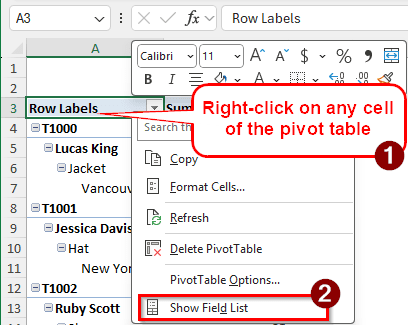
➤ Right-click on any cell of the pivot table.
➤ Select Show Field List
Although getting the menu back is easy, there is no obvious way to do it if you don’t know how. This tutorial will teach you how to show the menu if your pivot table field list is not showing. Learn both of the methods shown below and use the one that you like.
Getting the Pivot Table Menu Back in Excel Using Context Menu
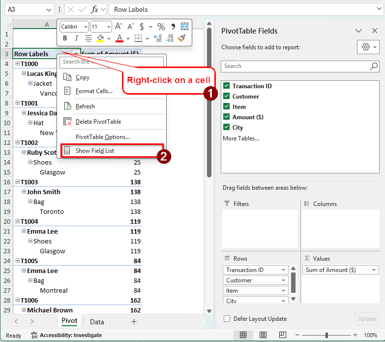
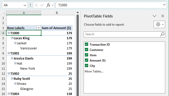
We have created a pivot table to show you how the fix actually works. In our pivot table, we have data about some retail transactions. There are transaction IDs, customer names, items, the amount of money the customers paid, and the cities where the products were delivered. However, after creating the pivot table, the “PivotTable Fields” section was closed. We need to get it back. Here is how to do it:
➤ In the pivot table, choose any cell. We are using an A3 cell for this one.
➤ Right-click on that cell to open the context menu.
➤ Click on Show Field List.
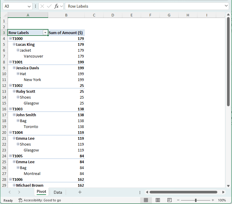
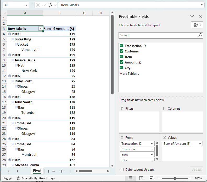
➤ Now the pivot table menu will show up.
Using the Ribbon Options to Get the Pivot Table Menu Back
The Ribbon in Microsoft Excel includes a lot of options that we can use to customize our worksheet. It also has the option to show the pivot table field list. Here is how we can use the ribbon to get the pivot table field list back:
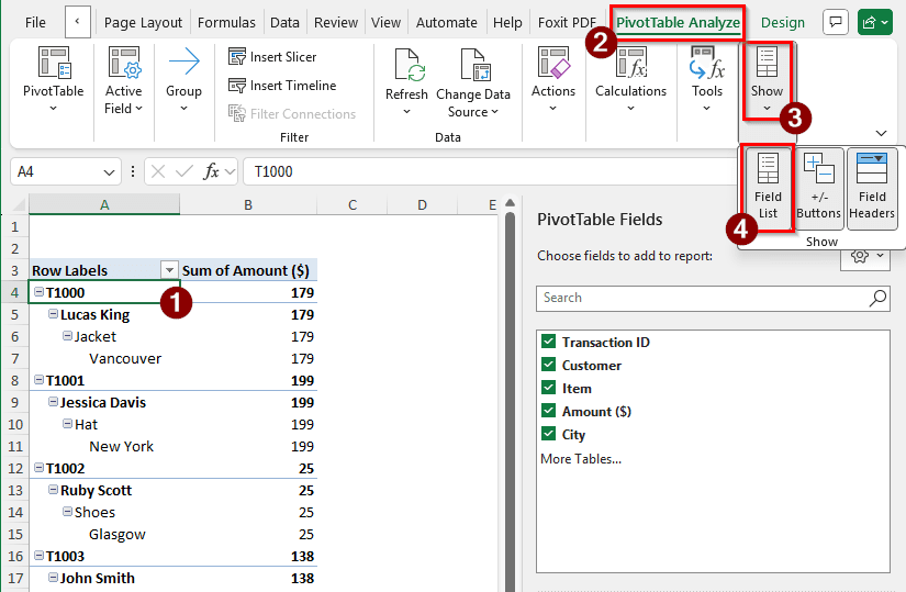
➤ Click on any cell of the pivot table. This will enable the PivotTable Analyze and Design tab in the ribbon.
➤ Go to the PivotTable Analyze tab.
➤ Find the section that says Show. It should be on the right of the pivot table.
➤ Click on Show List to make the pivot table menu show up.
Making Use of Keyboard Shortcuts to Get the Pivot Table Menu Back
Instead of using the GUI, we can make use of our keyboard to get the pivot table menu back. There are keyboard shortcuts for almost everything in Microsoft Excel. You can use keyboard shortcuts to cut the time you need to move your mouse from the pivot table. Moreover, you can keep working on the pivot table and keep everything in place while making sure that the pivot table field list pops up.
➤ Click on any cell of the pivot table. This is required to enable the pivot table and make changes.
➤ Assuming you are on the Home tab, press the following buttons sequentially. Remember, don’t press them together. Press them one by one.
Alt > J > T > L
➤ After this, the pivot table menu will show up. If the pivot table field list is already showing, it will be hidden.
Frequently Asked Questions
Why is the PivotTable option not showing up?
The pivot table options were probably closed for some reason. If the PivotTable Fields menu is closed for some reason, it will not show up even if you click and select a cell of the pivot table. You need to enable the options again to make sure that it shows up.
How do I add a PivotTable tab in Excel?
To do that, you need to insert a pivot table using your existing data. Don’t worry, your dataset will not vanish or be converted to something else permanently. Go to the Insert tab of the ribbon at the top, and select PivotTable. Set the data range and where you want your pivot table to show up, and hit OK. You might also want to add it to the data model if you need to do advanced data analysis.
How do I add a PivotTable to the Quick Access toolbar?
Right-click on the quick access toolbar and select “Customize Quick Access Toolbar”. A new window will pop up. In the left, from the “Choose commands from:” dropdown menu, select All Commands. Then, find PivotTable Tools in the left pane, select it, and click Add. This will add the panel to the right panel, which the quick access toolbar will use. Press OK to confirm.
How do you display a pivot table in Excel?
You need to create a pivot table in order to make it show up. It is possible to create a pivot table from any data range, whether it’s a table or not. Go to Insert > PivotTable to create a pivot table and display it in Excel.
How do I expand a PivotTable?
You can double-click on a cell of the pivot table to expand it. If you want to expand all the fields in the pivot table, right-click on the cell, go to Expand, and select “Expand Entire Field”.
Wrapping Up
In this article, we have learned how to get the pivot table menu back in Excel. We hope that having no PivotTable Fields will not restrict your data analysis activities anymore. If you want to read more Excel tutorials, bookmark our site and visit it whenever you encounter an issue working in Excel. Stay tuned for more Excel guides.