Pivot tables are often filtered with different criteria to understand the data better. When we put a filter on a pivot table, there is an arrow that shows up with the column header. If you want to use an image of the data in your presentation, the arrow with the column can confuse potential investors and managers who are not familiar with pivot tables. In this article, we will learn how to hide filter arrows in a pivot table so that you can make the table look cleaner.
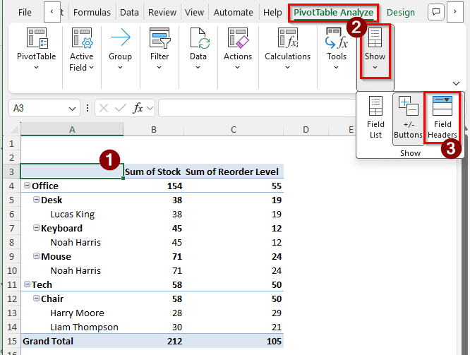
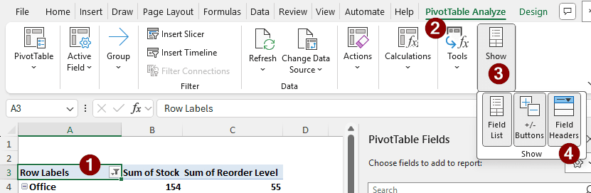
➤ Select a cell of the pivot table to activate the tabs related to the pivot table on the ribbon.
➤ Go to the PivotTable Analyze tab.
➤ In the Show group, deselect Field Headers.
Filter arrows can be annoying to deal with. In this article, we will learn three ways to hide filter arrows in your Excel pivot table. Download the Excel file we used in this tutorial to try the methods yourself.
Hiding Field Headers to Hide Filter Arrows
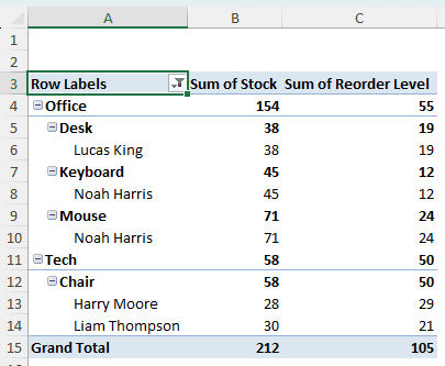
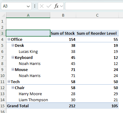
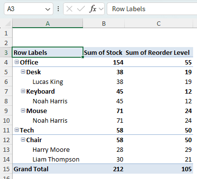
In order to demonstrate the ways you can hide filter arrows, we have prepared a dataset and a pivot table with that data. In our dataset, we have a few office supply items. There are item names, categories of the items, stock level of the products, the reorder level, and the supplier names. We have filtered the fields so that the Office and Tech items are visible, and not the Furniture items. However, the marker for the filter is visible on the pivot table. We need to hide that.
Pivot tables don’t have a direct option to hide the filter arrow. But we can hide the field headers in the pivot table to hide the filter arrows. This is essentially a workaround, but it is easy to implement and it works every time. Follow the steps below:
➤ First, move to a cell that belongs to the pivot table. This is needed so that we can use the PivotTable Analyze and Design tabs in the ribbon.
➤ Go to the PivotTable Analyze tab, and find the Show section.
➤ There should be three buttons that are selected. On the right, click on the Field Headers icon to deselect it.
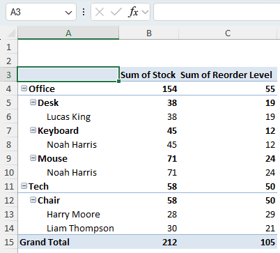
➤ Now the arrow in the A3 cell will vanish, along with the caption.
Disabling Field Captions and Filter Dropdowns to Hide Filter Arrows
In the settings of individual pivot tables, it is possible to disable field captions, which will remove the filter arrows. Here are the steps on how to do it:
➤ We can access pivot table options in two ways. First, we can right-click on a cell of the pivot table and select PivotTable Options.
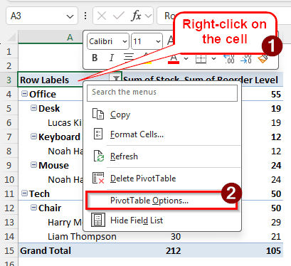
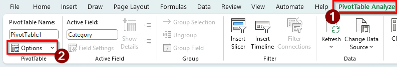
➤ You can also go to the PivotTable Analyze tab in the ribbon, and select Options from the PivotTable section.
➤ In the PivotTable Options window, head to the Display tab, and uncheck Display field captions and filter drop downs.
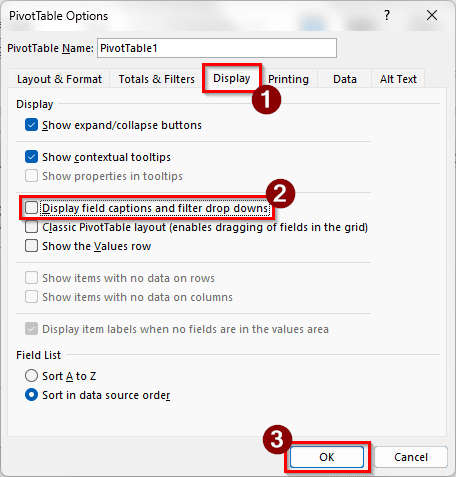
➤ Click on OK to save the change and see the results.
Using VBA to Hide Filter Arrows in Excel Pivot Table
Applying this method is harder than the previous two methods, but it is the best method to do the job. The reason behind that is that this method, unlike the other methods, does not remove the column labels. Instead, it just removes the filter arrows and makes the table look clean. Follow the steps below to apply this method to your dataset.
➤ While you are on the spreadsheet, press Alt + F11 to open the “Microsoft Visual Basic for Applications” window.
➤ Go to Insert > Module to open the code editor.
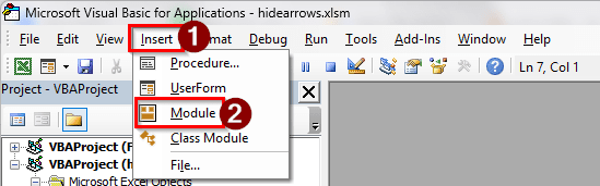
➤ Write the following code in the code editor:
Sub TogglePivotFieldSelection()
    Dim field As PivotField
    For Each field In ActiveSheet.PivotTables(1).PivotFields
        field.EnableItemSelection = Not field.EnableItemSelection
    Next field
End Sub
➤ Go to Run > Run Sub/UserForm to run the code.
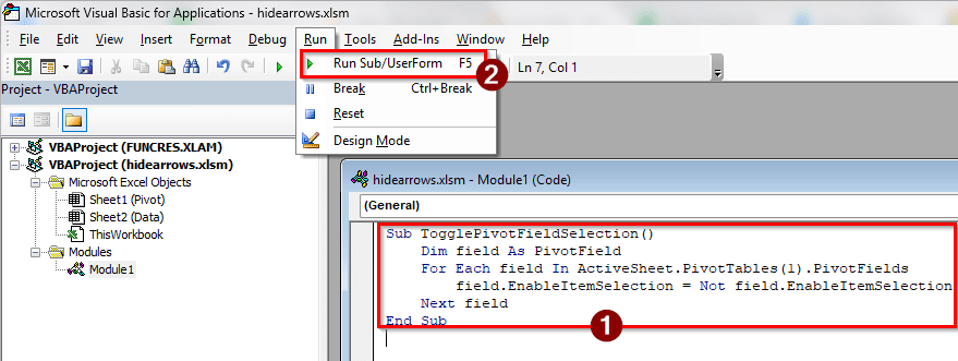
➤ Go back to your pivot table to see the results.
➤ You can run the code again to get the arrows back.
Frequently Asked Questions
How to get rid of dropdown arrows in an Excel table?
Select a cell of the Excel table to enable the Table Design tab. In the Table Style Options group, uncheck the box that says Filter Button. The dropdown arrows in the Excel table will be removed.
What is the difference between a slicer and a filter?
Slicer is a tool that allows you to filter data in the pivot table. However, the filters applied using a slicer aren’t permanent. Slicers are usually used to show filtered data in the pivot table for a quick view. Regular filters are applied for a more permanent solution, and the filtered table is used for further processing.
How do I remove the arrows in Excel?
If your cell is flagged with an error and shows a little arrow in it, it’s better to try to fix the issue. However, the arrow can show up without any errors as well. To remove this, go to File > Options. In the new window, go to the Formulas tab on the left. On the right, find the section that says Error Checking, and uncheck the box with the caption “Enable background error checking”. Press OK to save the settings.
How do I unsort a filter?
If you have just applied the filter, you can just Ctrl + Z to undo it and unsort the filter. If it has been a while, find the Editing group in the Home tab. Then, go to Sort & Filter, and click Clear from the dropdown menu.
How to convert a PivotTable back to raw data?
If you don’t have the source data anymore, change the pivot table layout to how you would want the source data to look. Then, select the whole range of the pivot table and copy by pressing Ctrl + C . Go to the new range where you want the data to be, and Paste Values from the Clipboard section of the Home tab.
Wrapping Up
In this article, we have learned how to hide filter arrows in a pivot table in Excel. Drop your feedback in the comment section below, and suggest what you want the next Excel tutorial to be about. We’ll be back with another article soon.