Filtering a table allows narrowing down a large set of data. If you have sales data for multiple regions, you would want to filter by different regions to get regional sales data. Moreover, you might want to put the sales representatives in another column and filter their data as well. Filtering columns with sales values may be needed to sort the target sales value.
While pivot tables allow doing all of that, there is no clear indication on how to do it. For a user who has never done this before, filtering multiple columns would possibly seem like a hassle. In this article, we will learn how to filter multiple columns in a pivot table in Excel.
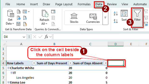
➤ Locate the row that contains the column labels in the pivot table.
➤ Select the column right beside the pivot table.
➤ Head to the Data tab in the ribbon, and go to the Sort & Filter group.
➤ Click on Filter. Now all the columns will have a filter dropdown that will allow you to filter multiple columns.
Filtering Multiple Columns with Values
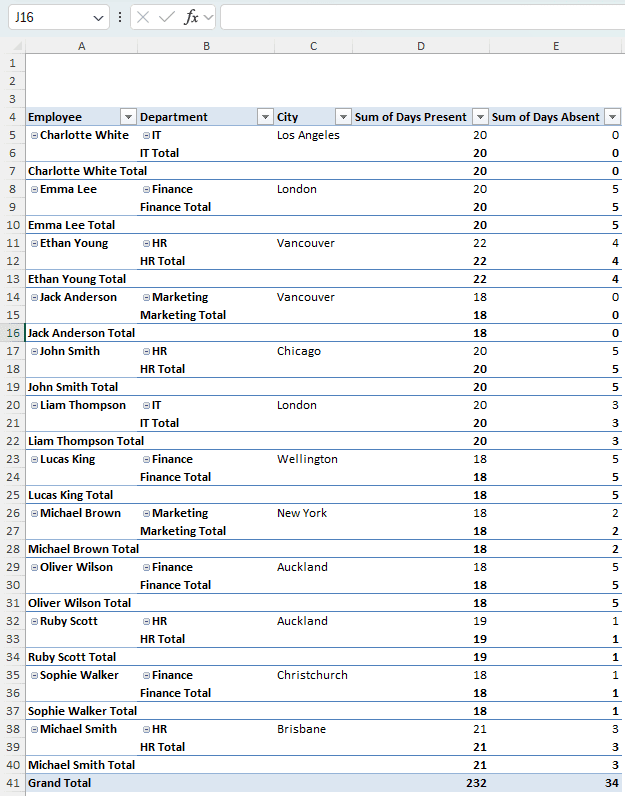
In order to demonstrate the methods, we have a pivot table with an employee attendance report. There are employee names, departments they work in, the number of days they were present and absent, and the cities they work in. We will put filters on the columns to check a specific number of present days. We will also filter the employees according to their departments to check department-wise attendance. Let’s begin:
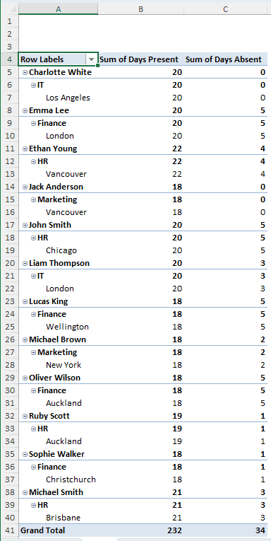
➤ In this table, the Row Labels cell has a dropdown menu that allows filtering the employees. However, we want to filter by the Sum of Days Present. It is a value field, and there are no dropdown menus for values.
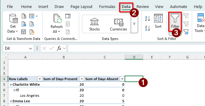
➤ To add one, go to the D4 cell as it belongs to the row that contains the column headings.
➤ Go to the Data tab in the ribbon, and find Sort & Filter.
➤ Click on Filter to add filter dropdowns to every column.
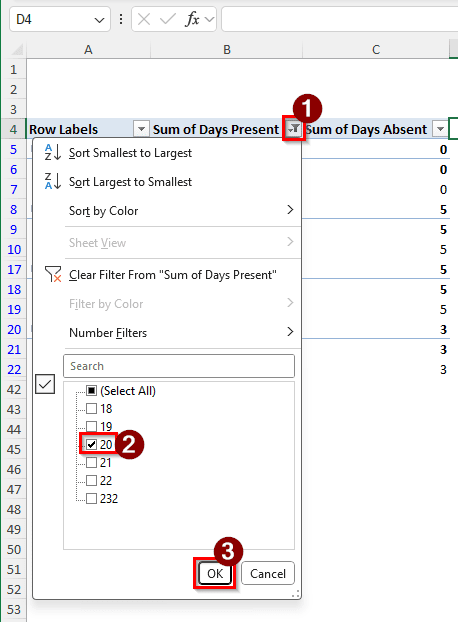
➤ Now we can filter multiple columns, including the columns that include values. For example, we can go to the dropdown menu of Sum of Days Present, uncheck Select All, and check 20. Pressing OK will filter the employees who were present for 20 days.
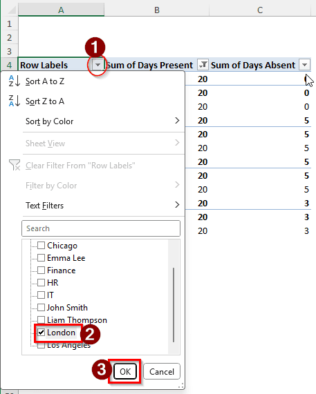
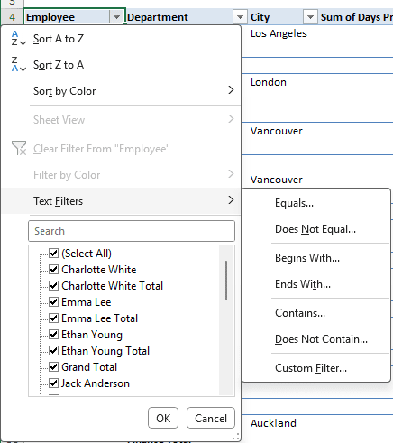
➤ Now go to the dropdown menu of A4, and select only the London checkbox.
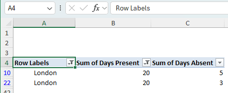
➤ After clicking OK, only the London rows will show up with their attendance.
Filtering Multiple Columns with Categories
We have added filters to value fields in the previous method. But what if we need filters for multiple columns with categories? The categories are shown in the same column in general. We need to show them in different columns to apply filters.
➤ Select any cell of the pivot table to activate the pivot table options in the ribbon.
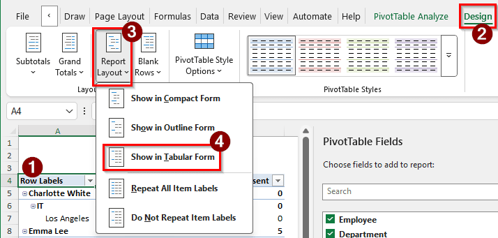
➤ Go to the Design tab. From the Report Layout button in the Layout group, select Show in Tabular Form.
➤ Now the pivot table allows filters for all the columns.
Adding Multiple Filters to Columns
By default, the columns only support one filter. We can filter the text from the context menu from the dropdown, but only one filter can be applied at a time. However, this restriction can be bypassed as well. Follow the instructions below:
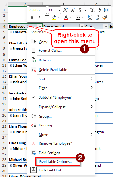
➤ Right-click on a cell of the pivot table, and select PivotTable Options from the context menu.
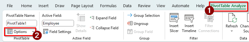
➤ You can also go to the PivotTable Analyze tab and select Options from the PivotTable group.
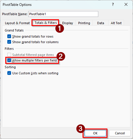
➤ In the PivotTable Options window, go to the Totals & Filters tab.
➤ In the Filters section, check the box that says Allow multiple filters per field. Press OK to confirm.
➤ Now we can select multiple filters from the dropdown menu.
Frequently Asked Questions
How to filter the top 10 values in PivotTable?
Right-click on the cell that you want to filter, then go to Filter > Top 10. A new window will open. Set the parameters of the filter in that window, and press OK.
Can you stack multiple filters?
Absolutely. In a pivot table, you can use multiple fields as filters. Just move the fields from the PivotTable Fields panel to the Filters area. A few cells with dropdown menus will be created at the top of the pivot table that will help you filter the data.
How to have a pivot table with multiple columns?
Usually, the pivot table will have values in the columns and the categories in the rows. If you want to show the categories in the columns, you can move the respective fields to the Columns section in the PivotTable Fields panel. If you don’t want to do that, you can use a layout for a pivot table that is anything but Compact.
How to create a pivot table in Excel?
Select the data range that you want to pivot, then go to the Insert tab of the ribbon. From there, select PivotTable. In the new window, press OK to create a pivot table in a new worksheet. If you want to do it in an existing worksheet, that option is available in that window as well.
How to group filter in a pivot table?
Select a cell of the field that you want to group in the pivot table. Right-click on that cell and select Group. A new window for grouping will pop up. Select the grouping options from that window and press OK to apply the grouping in the pivot table.
Wrapping Up
In this article, we have learned how to filter multiple columns in a pivot table. If you have followed the methods in this article properly, all of the columns in your pivot table can now be filtered, whether they contain values or categories. Additionally, we have learned how to apply multiple filters as well, which should help you filter the columns more accurately. Download the Excel file to practice the methods, and leave your feedback below.