Pivot Tables are mostly used for summarizing and analyzing data. But sometimes, a simple table is not enough to highlight the most important data. Conditional formatting lets you apply specific formats like colors, icons, or data bars to cells that meet certain criteria. This is also useful in a Pivot Table, as it can help you highlight important data.
In this article, we will walk you through two effective methods for applying conditional formatting in Pivot Table to make your data visually appealing.
To apply conditional formatting in Pivot Table, here is one simple solution by using the formatting icon.
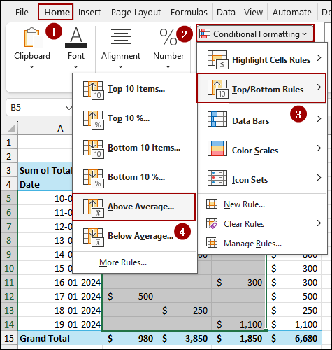
➤ Selecting cells click Home > Conditional Formatting > Top/Bottom Rules > Above Average.
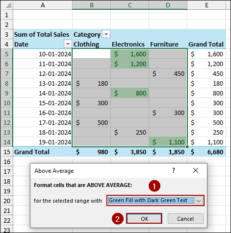
➤ From the dropdown menu, choose Green Fill with Dark Green Text and click OK.
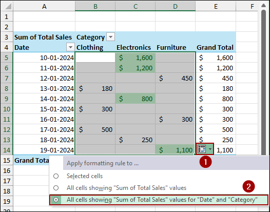
➤ Click the formatting icon and choose the third option: All cells showing “Sum of Total Sales” values for “Date” and “Category” to apply formatting in Pivot Table.

Using Pivot Table Formatting Icon
The quickest way to apply conditional formatting to a Pivot Table is by using the special formatting icon that appears when you apply a rule. This method applies the formatting correctly for the summarized data, even if the Pivot Table updates with new data.
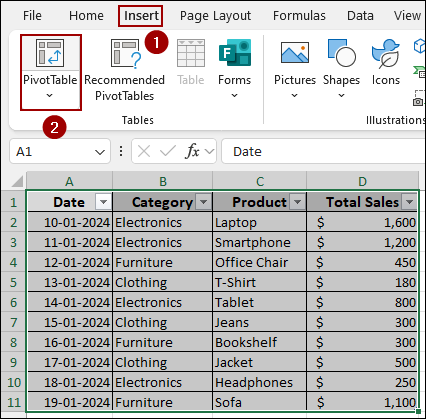
Suppose we have some sales data for various products and categories. We will start by creating a Pivot Table from this dataset.

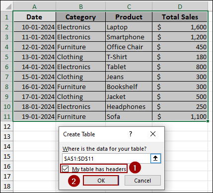
➤ Select the dataset and press Ctrl + T .

➤ In the Create Table dialog box, choose My table has headers and click OK to create the table.
➤ Now, with your data selected, click Insert > PivotTable.
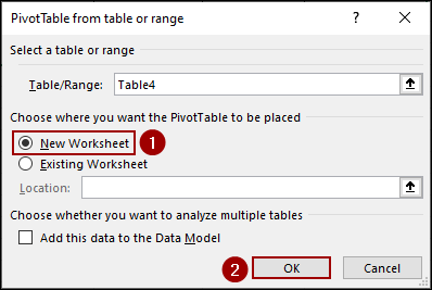
➤ In the new dialog box, choose New Worksheet and click OK to create your Pivot Table on a clean sheet.
➤ Drag the Date field to the Rows area, Category to the Columns area, and Total Sales to the Values area.
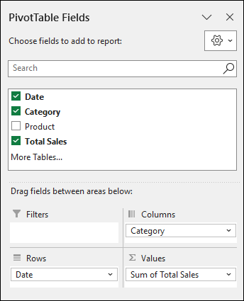
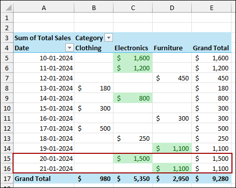
This will generate a Pivot Table showing total sales by date and category.

Now, let’s apply a conditional formatting rule to this Pivot Table to highlight sales that are above average.
➤ Choose cells from the Pivot Table.
➤ Go to the Home tab on the ribbon.
➤ In the Styles group, click Conditional Formatting.
➤ Hover over Top/Bottom Rules and select Above Average.
A new dialog box will appear.
➤ From the dropdown menu, choose Green Fill with Dark Green Text and click OK.
The Pivot Table will now have conditional formatting applied. Below, you will notice a formatting icon at the bottom right of the formatted cells.
➤ Click the icon to see your options.
➤ Choose the third option: All cells showing “Sum of Total Sales” values for “Date” and “Category”.
This ensures that the formatting rule applies correctly to all values within the Pivot Table, not just the selected cells.
If we add new data to your source table, the Pivot Table needs to be refreshed to update the conditional formatting. Here, we have added new rows of data to your original table.

➤ Right-click anywhere in the Pivot Table.
➤ From the context menu, select Refresh.
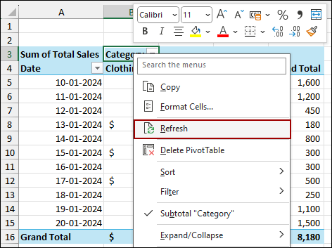
As a result, the Pivot Table will update to include the new data, and the conditional formatting will be applied to the new values automatically.
Applying New Rule from Conditional Formatting
For more advanced or custom conditional formatting, you can use the New Rule feature. This provides more control over the criteria and formatting style. Here, we will use the same Pivot Table as before and create a new rule to highlight all sales greater than $300.
➤ Select the sales values in your Pivot Table.
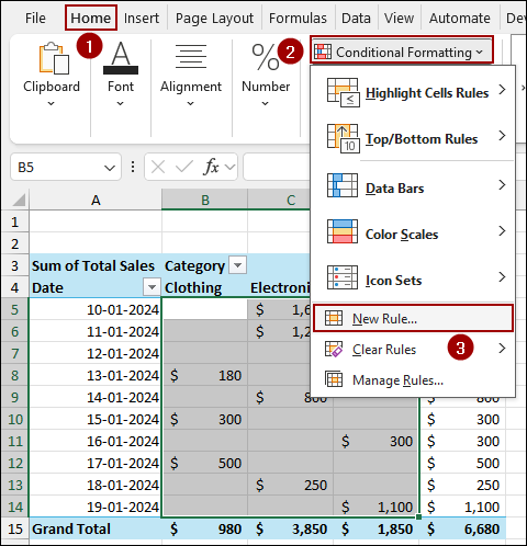
➤ Go to the Home tab and click Conditional Formatting.
➤ This time, select New Rule from the dropdown menu.
A dialog box will open.
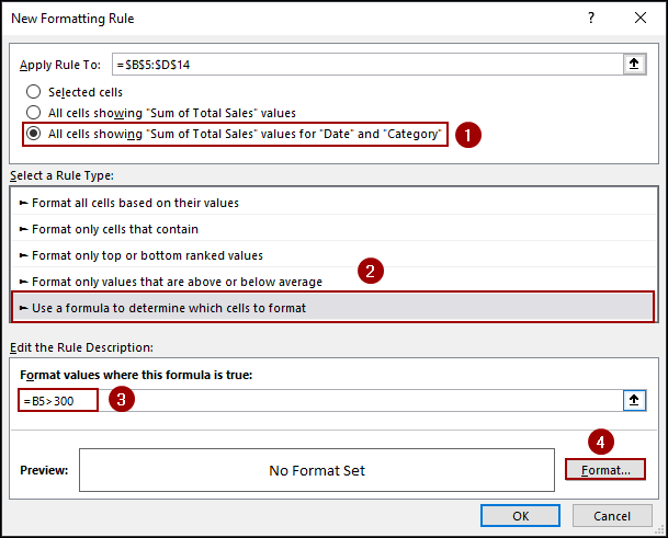
➤ Choose the option All cells showing “Sum of Total Sales” values for “Date” and “Category”.
➤ From the Select a Rule Type pane, choose Use a formula to determine which cells to format.
➤ In the Format values where this formula is true box, enter the formula
=B5>300
➤ Click the Format button.
➤ Go to the Fill tab.
➤ Choose your desired color, such as green, and click OK.

➤ Click OK again to apply the rule.

Finally, the Pivot Table will show a new conditional formatting rule, highlighting all sales values over $300 with a green fill.

Frequently Asked Questions
What is the main difference between using the formatting icon and a new rule?
The formatting icon gives you quick options for common rules (like Above Average or Top 10) and lets you easily apply the rule to the entire Pivot Table. Creating a new rule provides more control and allows you to use custom formulas.
Is it possible to apply different conditional formatting rules for different levels (Year vs Month) in a Pivot Table?
Yes, but you will need to create separate rules. For example, one rule for yearly totals, another for monthly details, and apply each to its respective fields.
Can I copy conditional formatting from one Pivot Table to another?
Yes, but only if both Pivot Tables share the same field structure. Use the Format Painter or copy/paste special > formats. Otherwise, you will need to reapply the rules.
Concluding Words
Above, we have discussed two simple ways to apply conditional formatting in a PivotTable. While the Pivot Table Formatting Icon is a quick option for highlighting values directly, creating a New Rule from the Conditional Formatting menu provides more formatting options. Depending on your needs, you can use either method to make your PivotTable more appealing. If you have any queries, feel free to let us know in the comments section below.