Combining Conditional Formatting with VLOOKUP function lets users dynamically highlight cells based on lookup results, making it easier to visually track matches. By using Excel’s built-in tools and functions, we can easily apply VLOOKUP based conditional formatting to highlight specific values across our dataset.
Follow the steps below to use Conditional Formatting based on VLOOKUP in your dataset.
➤ Start by selecting the range of cells where you want to apply conditional formatting.
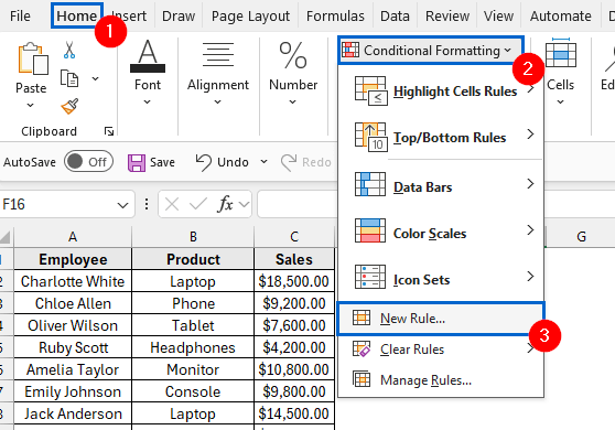
➤ Then, navigate to Conditional Formatting >> New Rule from the main menu.
➤ Click on Use a formula to determine which cells to format option and under Format values where this formula is true field, enter the following formula:
= [Cell1] < VLOOKUP([LookupValue], [LookupTable], [ColumnNumber], [MatchType])
➤ Replace [Cell1] with the value you want to compare against the lookup result.
➤ Replace [LookupValue] with the cell that contains the item you want to search for.
➤ Replace [LookupTable] with the range of cells that contains both the lookup values.
➤ Replace [ColumnNumber] with the number of the column in the lookup table that contains the result you want to retrieve.
➤ Replace [MatchType] with FALSE if you want an exact match or TRUE for an approximate one.
➤ Next, select a fill colour of your choice, and repeat the steps again to create another rule for values greater than or equal to your criteria.
In this article, we will learn how to apply conditional formatting based on VLOOKUP in three simple steps. We will also explore three alternative methods to achieve the same result.
Highlighting Matching Values Using Conditional Formatting & VLOOKUP
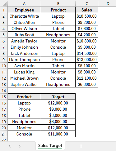
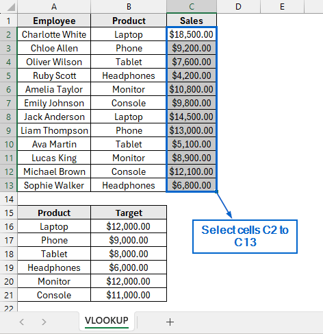
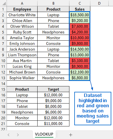
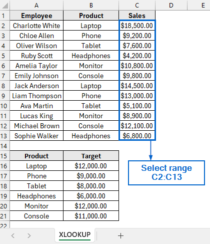
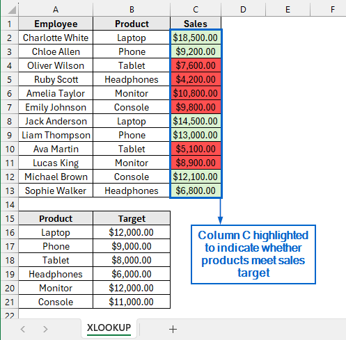
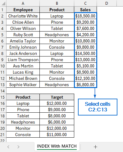
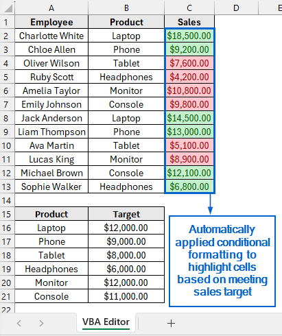
In the sample dataset, we have a worksheet containing information about Employee names, Product, Sales and Sales Target. Using conditional formatting with VLOOKUP, we will highlight the cells in red or green depending on whether they meet the sales target criteria. The updated dataset will be stored in a separate worksheet called “VLOOKUP”.
VLOOKUP is an important Excel function used to search for a value in one column and return a corresponding value from another column. Conditional formatting, on the other hand, is a feature that allows users to apply specific formatting to cells based on set conditions.
By combining these two, we can create dynamic formatting rules that highlight cells based on lookup results, making it easier to analyze and interpret data. Follow the steps below to correctly set up conditional formatting based on VLOOKUP to highlight cells in your dataset.
Step 1: Apply Conditional Formatting Rule to Highlight Sales Below Target
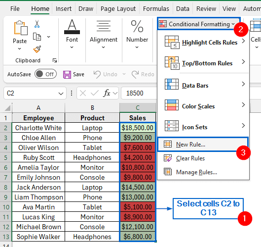
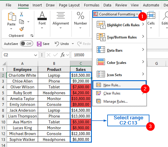
➤ Head to the VLOOKUP worksheet and select cells C2 to C13.
➤ From the main menu, navigate to Conditional Formatting >> New Rule.
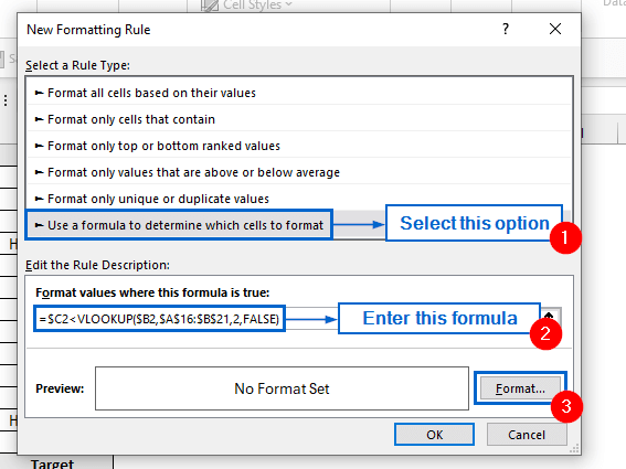
➤ In the New Formatting Rule dialogue box, choose the option Use a formula to determine which cells to format. Next, type the formula into the Format values where this formula is true box and click Format.
=$C2<VLOOKUP($B2,$A$16:$B$21,2,FALSE)
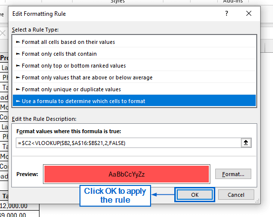
➤ Next, in the Format Cells dialogue box, go to the Fill tab, choose a red colour, and click OK.

➤ Finally, click OK in the New Formatting Rule dialogue box to apply the formatting rule.
Step 2: Apply Conditional Formatting Rule to Highlight Sales Meeting or Exceeding Target
➤ Go to the dataset again, select the range C2:C13, then head to Conditional Formatting >> New Rule.
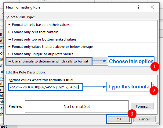
➤ Select Use a formula to determine which cells to format option, enter the following formula under Format values where this formula is true field and click on Format.
=$C2>=VLOOKUP($B2,$A$16:$B$21,2,FALSE)
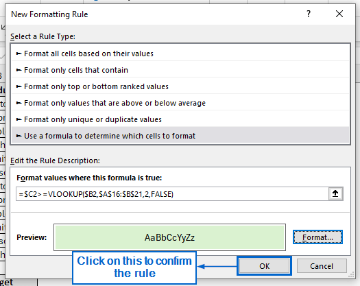
➤ Next, go to the Fill tab, pick a green colour and select OK.

Step 3: Finalize the Rules and Display the Highlighted Results
➤ Now, click on OK from the New Formatting Rule dialogue box to complete the process.
➤ The dataset should now highlight products that meet the sales target in green, and those that don’t in red.
Alternative Methods to Apply Conditional Formatting Based on Lookup Value
While the VLOOKUP function is often used to apply conditional formatting based on a lookup value, it has certain limitations. For example, it only looks from left to right and requires the lookup column to be the first in the table array.
Alternative methods, such as the XLOOKUP function, the INDEX-MATCH combination, and the VBA Editor, provide greater flexibility and handle datasets more efficiently.
Use XLOOKUP for Flexible Conditional Formatting
XLOOKUP is an advanced Excel function that searches for a value in a range or array and returns the corresponding result from another range. Unlike VLOOKUP, it can look both to the left and right, offering greater flexibility in handling datasets.
Using the same dataset, we will now apply conditional formatting with the XLOOKUP function to highlight cells in green for values that meet the criteria and in red for those that do not. We will display the modified dataset in a separate “XLOOKUP” worksheet.
Steps:
➤ Head to the XLOOKUP worksheet and select range C2:C13.
➤ Go to Conditional Formatting >> New Rule from the main menu.

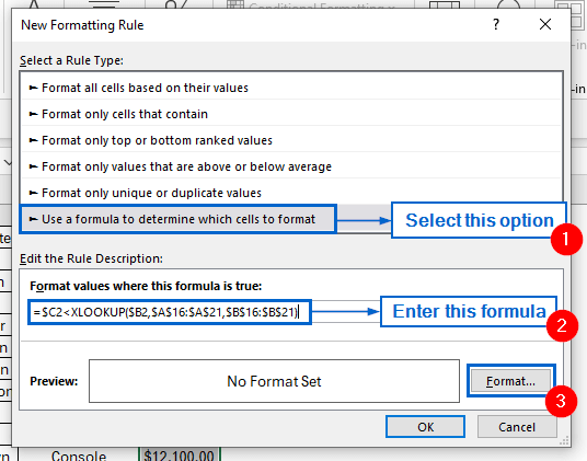
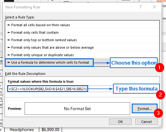
➤ In the New Formatting Rule dialogue box, select Use a formula to determine which cells to format option and enter the formula below in the field provided, then click Format.
=$C2<XLOOKUP($B2,$A$16:$A$21,$B$16:$B$21)
Note:
This formula works the same way as the previous method, but uses XLOOKUP to look for the matching value in the reference table and highlight cells where the value in C2 is smaller than that lookup result.
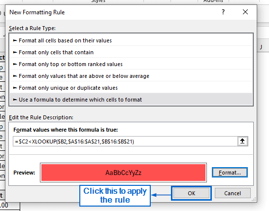
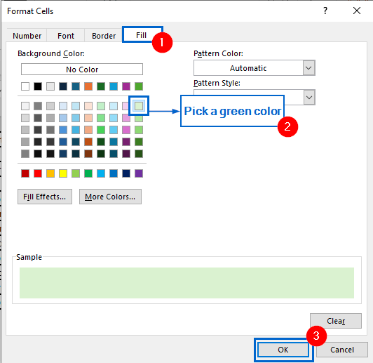
➤ In the Format Cells window, head to the Fill tab, choose a red fill colour, then click OK.

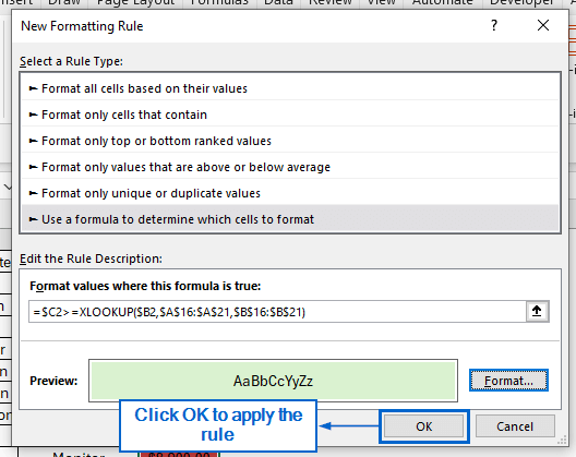
➤ Click OK in the New Formatting Rule dialogue box to apply the formatting rule.
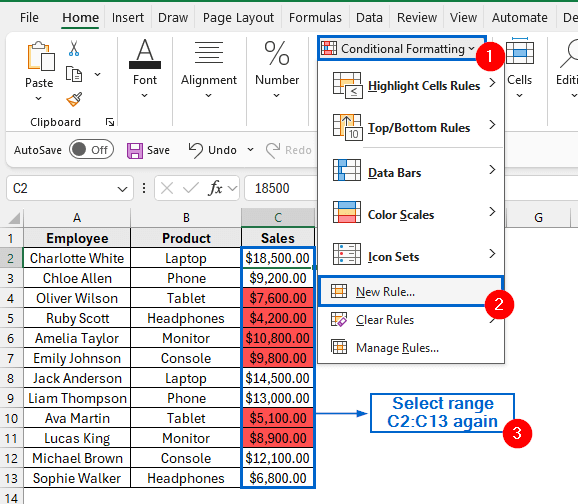
➤ Select cells C2:C13 again, and head to Conditional Formatting >> New Rule.
➤ Choose Use a formula to determine which cells to format option, enter the formula below, then click Format.
=$C2>=XLOOKUP($B2,$A$16:$A$21,$B$16:$B$21)
➤ Head to the Fill tab again, apply a green fill colour and press OK.
➤ Click OK to complete the operation.
➤ The worksheet will now highlight items that meet or exceed the sales target in green and red, respectively.
Apply Conditional Formatting with INDEX and MATCH Functions
The INDEX function in Excel is used to return value of a cell within a specified range, while MATCH is used to find the relative position of a value within a range. By combining these two functions and applying conditional formatting, we can easily highlight cells that meet specific conditions.
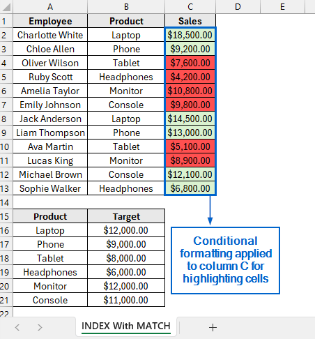
Working again with the same dataset, we will now apply conditional formatting using the INDEX and MATCH functions to highlight the dataset based on a specific lookup value. We will display the updated dataset in a separate “INDEX With MATCH” dataset.
Steps:
➤ Head to the INDEX With MATCH worksheet and select cells C2:C13.
➤ From the main menu, select Conditional Formatting >> New Rule.

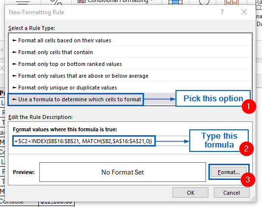
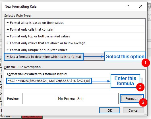
➤ In the New Formatting Rule window, choose Use a formula to determine which cells to format option. Type the formula below into the input box, then click Format.
=$C2<INDEX($B$16:$B$21, MATCH($B2,$A$16:$A$21,0))
Note:
Similar to the first method, this formula uses INDEX and MATCH functions to check whether the sales value in cell C2 is less than the target value and highlights the cell accordingly.
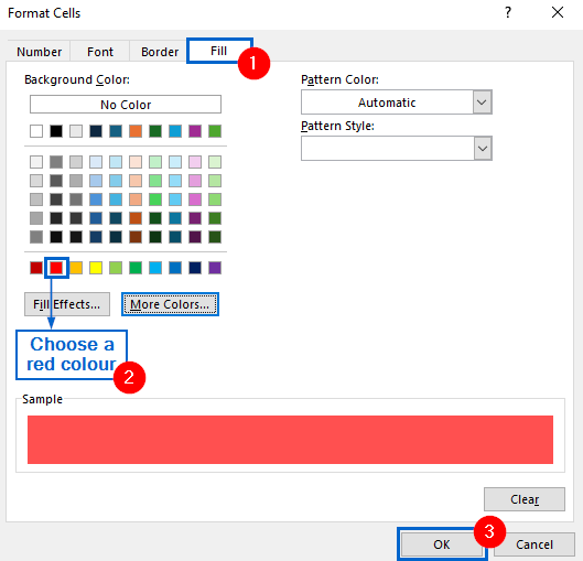
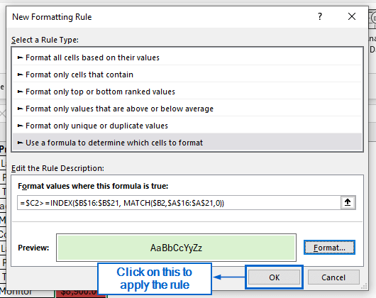
➤ Go to the Fill tab from Format Cells dialogue box, select a red fill colour and press OK.
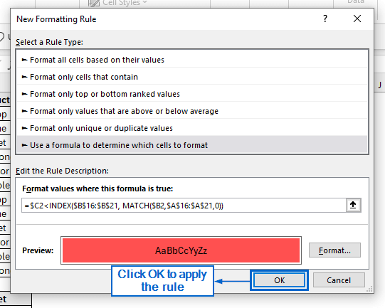
➤ From the New Formatting Rule dialogue box, click OK to apply the formatting rule.
➤ Head to the dataset again, select range C2:C13 and head to Conditional Formatting >> New Rule.

➤ Pick Use a formula to determine which cells to format option, enter the following formula in the box, and click Format.
=$C2>=INDEX($B$16:$B$21, MATCH($B2,$A$16:$A$21,0))
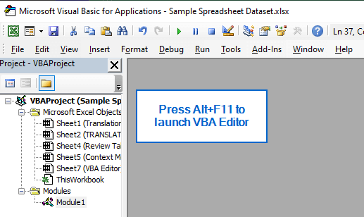
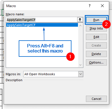
Note: ➤ Go to the Fill tab again, choose a green colour, then press OK to confirm selection. ➤ Click OK again to finally apply the rules. ➤ Column C should now highlight cells in red and green depending on whether each product has met its defined sales target. VBA Editor is a powerful Excel tool that enables users to write custom macros and automate repetitive tasks, saving time and effort. Working with the same dataset again, we will now apply conditional formatting using the VBA Editor to highlight the Sales column based on whether they meet the defined targets. We will display the modified dataset in a separate worksheet called “VBA Editor”. Steps: ➤ Go to the VBA Editor worksheet and press Alt + F11 to open the VBA Editor window. ➤ Next, from main menu, head to Insert >> Module and paste the following script. ➤ Now, close the VBA window, press Alt + F8 to open the Macros dialogue box, select the ApplySalesTargetCF macro, and click Run. ➤ You should now see cells in the Sales column highlighted in green and red based on whether the sales target is met. For large datasets, the XLOOKUP or INDEX+MATCH methods are the best options since they allow lookups in both directions. The VBA Editor is also efficient for large datasets, as it can automate formatting across the entire range with a single macro. To highlight the entire row using VLOOKUP, you need to apply conditional formatting to the whole row range and adjust the formula so it references the lookup value for that row. Knowing how to use conditional formatting based on VLOOKUP is essential for quickly highlighting key data and performing efficient data analysis. In this article, we have discussed four effective methods of applying conditional formatting based on VLOOKUP, including using the VLOOKUP function, XLOOKUP function, combining INDEX with MATCH function and VBA Editor. Feel free to try out all methods and choose the one that best fits your needs.
This formula checks whether the sales value in cell C2 is greater than or equal to the target value and highlights the cell if the condition is met.
Automate Conditional Formatting with VBA Editor
Sub ApplySalesTargetCF()
    Dim ws As Worksheet
    Dim rng As Range
    Set ws = ActiveSheet
    ' Range of Sales values to format
    Set rng = ws.Range("C2:C13")
    ' Clear existing conditional formatting on column C
    rng.FormatConditions.Delete
    ' Green rule: Sales >= Target
    With rng.FormatConditions.Add(Type:=xlExpression, _
        Formula1:="=$C2>=VLOOKUP($B2,$A$16:$B$21,2,FALSE)")
        .Interior.Color = RGB(198, 239, 206)   ' light green
        .Font.Color = RGB(0, 97, 0)            ' dark green text
    End With
    ' Red rule: Sales < Target
    With rng.FormatConditions.Add(Type:=xlExpression, _
        Formula1:="=$C2<VLOOKUP($B2,$A$16:$B$21,2,FALSE)")
        .Interior.Color = RGB(255, 199, 206)   ' light red
        .Font.Color = RGB(156, 0, 6)           ' dark red text
    End With
       MsgBox "Conditional Formatting applied to Sales column based on Targets!"
End Sub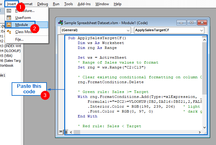
Frequently Asked Questions
Which Method Should I Use For Large Datasets?
How do I Highlight the Entire Row Instead of a Single Cell with VLOOKUP?
Concluding Words