
Manually scanning through a long list of data and finding a specific value or text is not a joke. It can be a more hectic task than you can think of. Whether you need to manage any project, track employee logs, or monitor inventory management, there are times when it is necessary to search for values based on text. Luckily, Excel is built and programmed for such narrow ends, too. It comes with an array of formulas to help you find in several different ways.
To count cells having specific text in Excel, you can follow these steps using the COUNTIF formula –
➤ In the datasheet, write a row with an appropriate header to store the number of times a text appears.
➤ Select the cell and write the following formula –
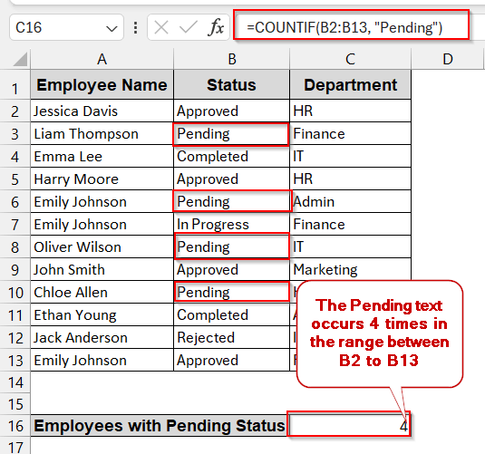
=COUNTIF(B2:B13, “Pending”)
where B2:B13 is the range containing the text value, and ‘Pending’ is the text that needs to be counted.
➤ Press Enter, and the result will return the number of times the text appears.
In this article, we will explore the ins and outs of the Excel methods for counting cells with specific text. Including exact matches, partial matches, case-sensitive matches, and multiple text criteria, there will also be automated results of the VBA approach. So, stay tight and go through each of them properly as we discuss all these methods in pinpoint detail.
Count Cells with a Specific Word Using COUNTIF
This method is the most beginner-friendly and is mostly used when finding words with an exact match. When going through statuses, logs, and categories tracking in product lists, COUNTIF works best. The best part is that it is case-insensitive and does not require you to maintain any cases.
For the methods, we will be using the following dataset. We will be counting how many times the text ‘Pending’ occurs.
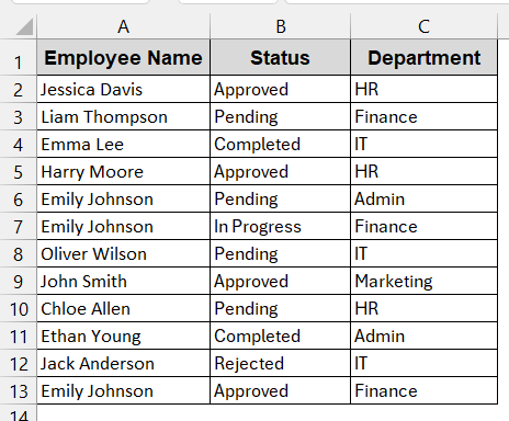
➤ Open the Excel sheet and locate the range of cells that have the texts you need to count. Here it is, B2 to B13.
➤ Make a new row to store the result, with an appropriate header, below the datasets.
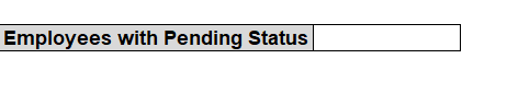
➤ Type the COUNTIF formula in the empty cell.
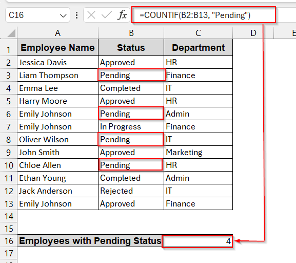
=COUNTIF(B2:B13, "Pending")
Here, B2:B13 is the cell range and ‘Pending’ is the text that we want to count.
➤ Press Enter, and you will get the result.
Notes:
➨ Ensure the spelling is correct and has no typos. Incorrect spelling or extra spaces will not give the expected output.
➨ You can also modify the formula by using the cell references instead of using the exact text –
=COUNTIF(B2:B13, B3),
where B3 is the cell that contains the text ‘Pending’.
Using COUNTIF with Wildcards for Partial Text Matches
Sometimes, we don’t want to find the exact text matches and go for the partial ones. For example, you might want to count the cells containing the text ‘end’ instead of ‘Pending’. In that case, you can modify the COUNTIF formula. With this, you can get the partial text match inside the cell, even it is a part of another text.
For this method, we will find the partial text ‘ed’ from the column Status.
Steps:
➤ Open the Excel sheet and find the range of the cells where you need to find the data (e.g, B2 to B13).
➤ Make a new row to store the value with the appropriate header.
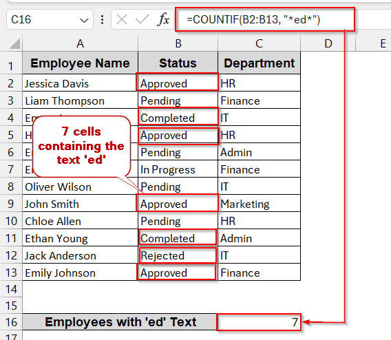
➤ Type the COUNTIF formula with the wildcards in the empty cell –
=COUNTIF(B2:B13, "*ed*")
Here B2:B13 is the range from which the text match of ‘ed’ needs to be counted.
➤ Press Enter to get the number of cells containing the partial text match. Here it is 7 for this dataset.
Notes:
You can also use the wildcard ‘?’ instead of ‘*’ to match the characters. For example, B?nding will count the cells having both Binding and Bonding (any character in the place of the wildcard).
Count Texts Based on Multiple Text Conditions with COUNTIF
Let’s be real; in the real world, we rarely find text with specific or partial text alone. While dealing with large datasets, we often need to find the texts based on multiple conditions. To be simple, we might need to count cells with the text ‘Pending’ and belonging to the ‘HR’ department. This can also be done with COUNTIF, which just modifies some parameters.
This method will count cells with the text ‘Pending’ in the Status column and ‘HR’ in the Department column.
Steps:
➤ Open the Excel workbook and locate the cell ranges with text matches. Here, it is B2 to B13 and C2 to C13.
➤ Make a row to store the result of the cell count, like before.
![]()
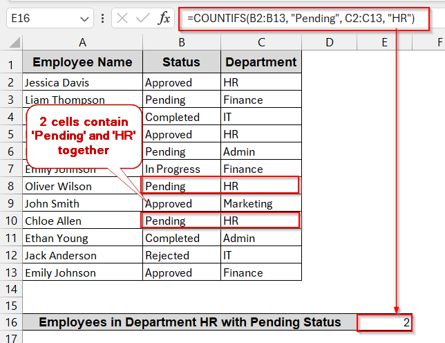
➤ Write the COUNTIF formula for multiple text matches –
=COUNTIFS(B2:B13, "Pending", C2:C13, "HR")
Here B2:B13 is the range of the cells containing ‘Pending’ and C2:C13 contains the range of cells containing ‘HR’.
➤ Press Enter to get the result in the empty cell, which is two here.
Notes:
➨ This COUNTIF function only counts the cells when all the conditions are met inside the parameter.
➨ It is also non-case-sensitive.
Counting Case-Sensitive Texts Using SUMPRODUCT and EXACT
The COUNTIF formula works best in almost every situation if you don’t need case-sensitive values. However, when you need to find the exact match along with case-sensitivity, you need to use the formulas of SUMPRODUCT and EXACT.
Here, in this method, we will be counting cells containing ‘pending’ text where all letters are in lowercase.
Steps:
➤ Open the Excel sheet and find the cell range that contains the text matches (e.g, B2 to B13).
➤ Create a new row to store the value of the result of the cell counts.
![]()
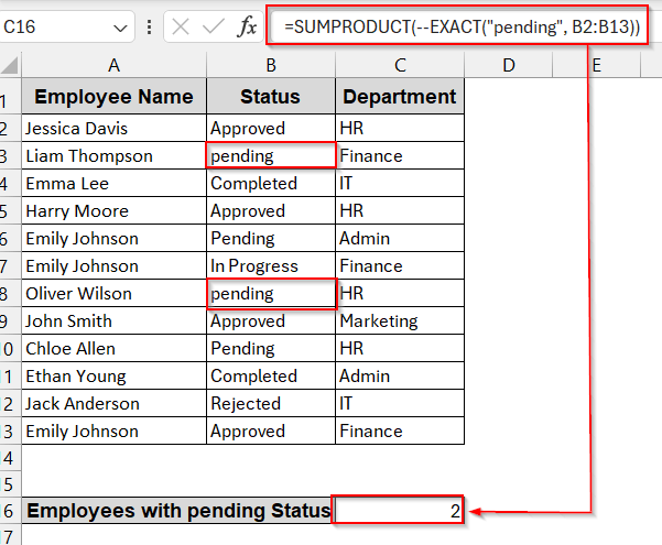
➤ Use the SUMPRODUCT+EXACT formula in the empty cell of the newly created row.
=SUMPRODUCT(--EXACT("pending", B2:B13))
➤ Press Enter to get the cell count result, which is two here.
Notes:
➨ The EXACT function is case-sensitive and, wrapped in —, makes it suitable for counting.
➨ This formula approach works best for the cell range containing the text value instead of numeric ones.
Count Text Matches in Excel 365 with FILTER Function
For Excel 365 users, counting text matches is a lot easier and more dynamic. You can use FILTER, COUNTA, and even SEARCH functions to count a certain word or part of it. As dynamic referencing is used, the result is automatically modified when the search word is changed.
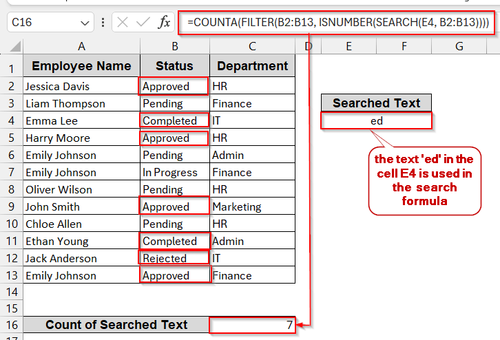
In this method, we will search for the text ‘ed’ by combining these three formulas.
Steps:
➤ Open the dataset and find the cell range to match the text.
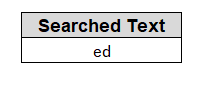
➤ Pick an empty cell and write the exact text you want to count. You can also give it an appropriate header.
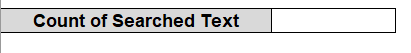
➤ Create another row to store the result of the cell count, like the previous example.
➤ Write the formula below in the empty cell –
=COUNTA(FILTER(B2:B13, ISNUMBER(SEARCH(E4, B2:B13))))
Here B2:B13 is the cell range and E4 is the cell containing the searched text.
➤ Press Enter to get the result in the desired cell.
Notes:
➨ SEARCH, just like COUNTIF, is not a case-sensitive formula. For case-sensitive values, you need to use the FIND function.
➨ Wrap the FILTER function in IFERROR to avoid #CALC! Error when no matched text is found.
Automated Text Matching in Excel Using VBA
When you need to use text matching several times, you can create a custom VBA-based formula. It is better and faster. As much as it automates the process , it also makes the sheet interactive by displaying the texts in a message box or cells.
Here, like before, we will find the text matches for the ‘Pending’.
Steps:
➤ Go to the Developers Tab and click on Visual Basic.
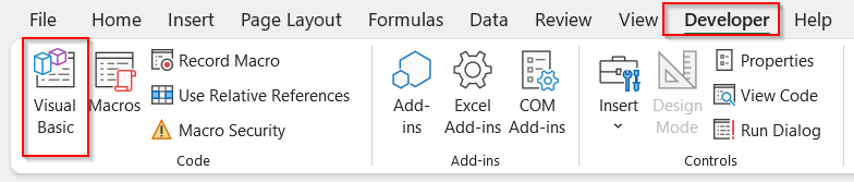
➤ This will launch the VBA editor window.
➤ Click on Insert and choose Module to write the VBA script.
➤ Paste the following code in the blank space below –
Function CountText(rng As Range, txt As String) As Long

    Dim cell As Range
    Dim count As Long
    count = 0
    For Each cell In rng
        If InStr(1, cell.Value, txt, vbTextCompare) > 0 Then
            count = count + 1
        End If
    Next cell
    CountText = count
End Function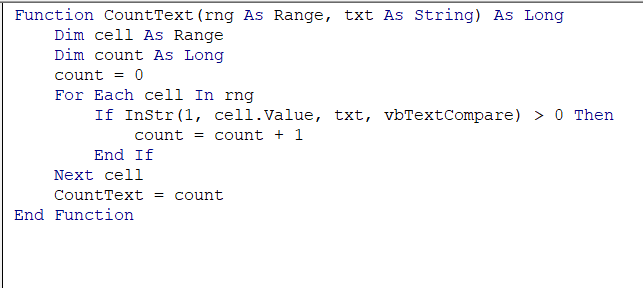
➤ Save the script by Ctrl + S and close the VBA editor.
➤ Create a new row to store the count of text matches.
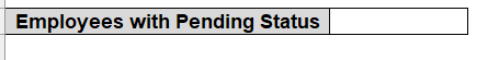
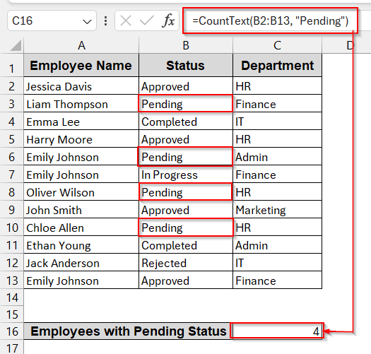
➤ Type the newly customized VBA formula in the blank cell.
=CountText(B2:B13, "Pending")
where CountText is the formula we created using VBA (see the first line of the VBA script) and ‘Pending’ is the text match in the range B2:B13.
➤ Press Enter to get the result in the desired cell.
Notes:
➨ The above VBA script is not case-sensitive due to the use of functions like InStr and vbTextCompare. To enable case sensitivity, change vbTextCompare to vbBinaryCompare in line 6.
If InStr(1, cell.Value, txt, vbTextCompare) > 0 Then
➨ This formula also enables wildcards for partial matches.
Excel Formula to Exclude Numbers and Blanks When Counting Text
In the practical dataset, a few columns contain only the text values. The columns can have a combination of data types, like numbers and blank cells. A generic method is not suitable for excluding non-text and blank cells. The best bet is to use ISTEXT along with SUMPRODUCT.
We have changed our data, replacing many values with blanks and numeric ones.
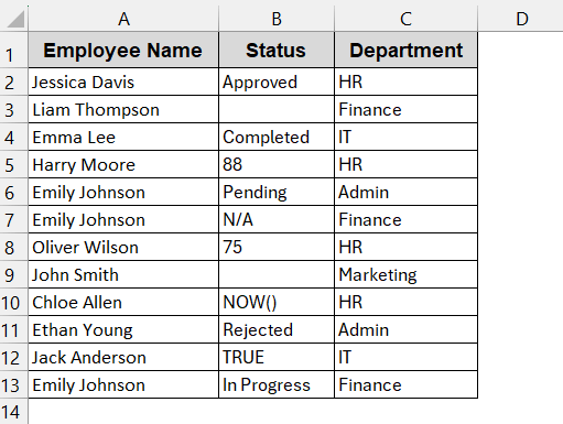
In this method, we will be counting cells that have only text values.
Steps:
➤ Create a row to store the result like before.
![]()
➤ Identify the range that you want to count.
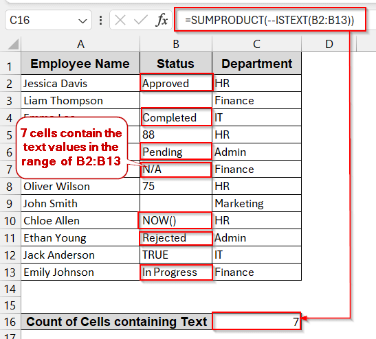
➤ Type the formula in the blank cell –
=SUMPRODUCT(–ISTEXT(B2:B13))
Here, B2:B13 is the range, and ISTEXT only filters cells that have text.
➤ Press Enter to get the result in the output cell.
Notes:
➤ If you want to count non-text cells, modify the NOT formula to ISTEXT –
=SUMPRODUCT(–NOT(ISTEXT(B2:B13)))
Frequently Asked Questions (FAQs)
What will COUNTIF still work if my text has trailing spaces?
The COUNTIF matched the exact and the partial text. Though case-insensitive, it does not work for typo mistakes and extra spaces. Even if you have trailing spaces in the text, the COUNTIF function will not work.
How can I count cells that contain one of several words?
If you want to count cells containing one of several words, a single COUNTIF function will not work. You can use separate COUNTIF functions for each word and add them up, or use SUMPRODUCT.
Can I make COUNTIF case-sensitive without using VBA?
You can’t make the COUNTIF function case-sensitive without using any external VBA script. The best way is to use the SUMPRODUCT and EXACT formula.
Why is my COUNTIF formula returning 0 when I have matching text?
The COUNTIF formula might not work even if you have matching texts due to spelling mistakes and extra spaces. Also, check the cell ranges if they are correct. Avoid copying text in the formula, as formatting issues can change the result.
How can I apply the COUNTIF formula across multiple sheets automatically?
To apply the COUNTIF formula across multiple sheets, combine it with SUMPRODUCT and INDIRECT formulas. Use the formula below –=SUMPRODUCT(COUNTIF(INDIRECT(“‘”&SheetNameRange&”‘!RangeToCount”), Criteria)).
Here, the SheetNameRange is the range that contains the sheet name, RangeToCount is the selected range from which the text will be counted, and Criteria is the text.
Concluding Words
Whether you are working with the project statuses, survey data, or the product category, Excel has its own set of powerful methods and tools to count cells with specific text. Starting from the basic COUNTIF, you can upgrade your results using SUMPRODUCT, EXACT, FILTER, and even automated VBA. As you understand how each method works and when to use it, you not only save time but also build smarter and interactive sheets. Download our workbook, try each method in your file, and see which is best for you.