Numbers are what the data speaks. But raw digits without units, suffixes, or prefixes hold no meaning. Imagine having an invoice with a column that reads just numbers. It is impossible to know if it states price, weight, or units. You can have meaningful headers, but without adding text to numbers, your Excel sheet remains lifeless and, more importantly, unprofessional. Keeping your numbers intact and without converting them to text, you can easily custom-format the cells to add text. It is easier, understandable, and keeps your sheets cleaner.
To custom format cells to add text after numbers, follow these simple steps.
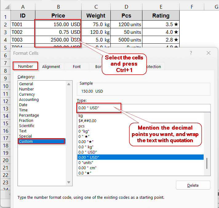
➤ Open the dataset and select the cells you want to format.
➤ Press Ctrl + 1 or right-click to select Format Cells.
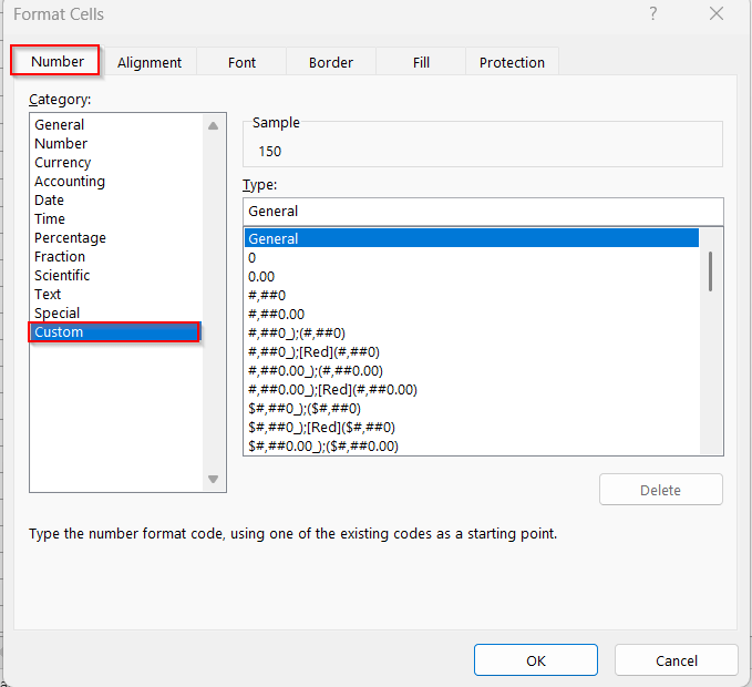
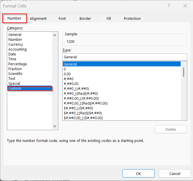
➤ In the Format Cells window, go to the Number tab and click on Custom in the Category.
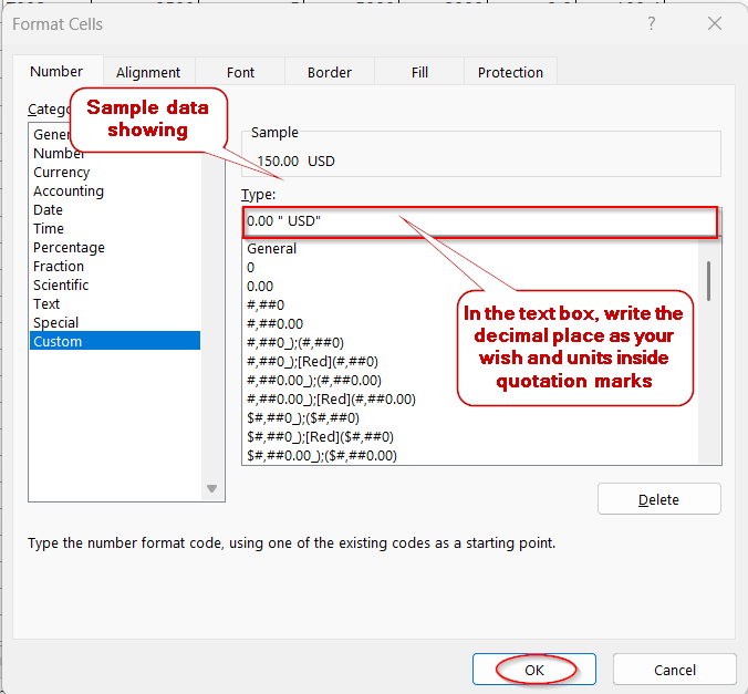
➤ In the Type text box, write the decimal place you want and the unit enclosed in quotation marks.
For example, to convert to kilograms with one decimal place, write- 0.0 “ kg” or use 0.00 “ USD” for currency.
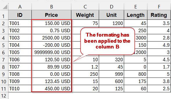
➤ Click OK to see the formatting of the cells.
There are various ways in which you can customize the format to add text after a number in Excel. You can add simple suffix/prefix, create conditional suffixes of positive, negative, or text sections, and scale greater numbers. Apart from that, there are also options to add special characters and symbols. Lastly, for more professional and advanced cases, you can opt for VBA solutions. So, dive in with us, and pick the one that fits with your datasheet and workflow.
Add Suffix Text with Numbers Using Custom Format
One of the most common scenarios is showing the units and their numbers. Though Excel has Format Cells options for most units, you might still struggle to find common ones like kilogram, centimeters, etc. Adding simply these units as texts makes the values non-numeric. As a result, you can use them to further calculations. In such cases, you can use the Custom Format of the Format Cells option to create these units.
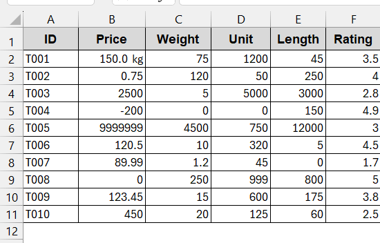
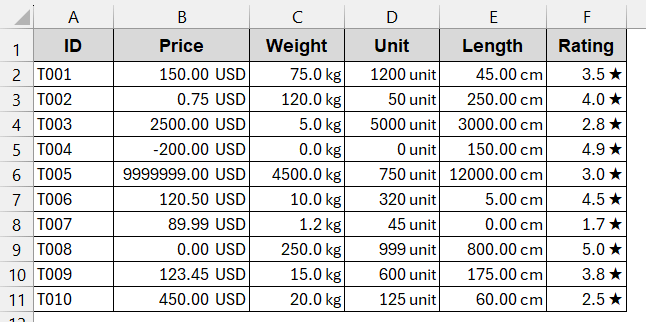
We will use the dataset below and add units accordingly for each column.
Steps:
➤ Open the dataset and see the cells needing custom formatting. In this example, we need to format all the columns, including Price, Weight, Unit, Length, Rating, and Temp.
➤ Select the cells of column B (Price), and press Ctrl + 1 to open Format Cells. You can also right-click and select Format Cells.
➤ In the Format Cells, go to the Number tab and choose Custom from the Category.
➤ In the Type box, write the decimal points, followed by the unit inside quotation marks –
0.00 “ USD”
➤ Click OK to apply the change to the column.
➤ Do the same for the rest of the columns.
➤ For column C, we used – 0.0 “ kg”
➤ For column D, we used – 0 “ units”
➤ For column E, we used – 0.00 “ cm”
➤ For column F, we used – 0.0 “ ★”
➤ At the end, the final dataset will look like this-
Notes:
You can add decimal places for precision. Without decimal places, all the values will be in whole numbers.
Conditional Suffixes for Positive, Negative, Zero & Text Sections
When preparing financial documents, not only does your Excel data need to have a suffix text, it also needs to have text to differentiate them visually. For example, we might need to add texts in the same column or cells, based on the positive or negative values. In this case, custom formatting isn’t enough – what you need is conditionals inside your customized formatting. In the custom formatting option, you can also give conditions to get different texts for different types of values and even strings.
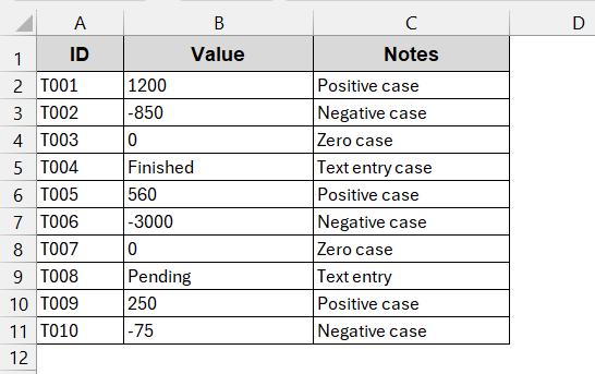
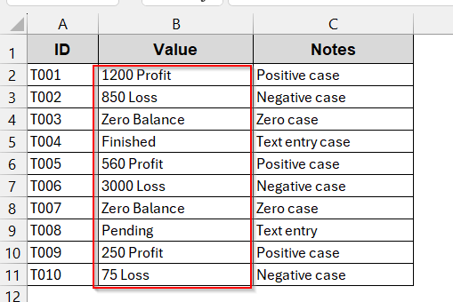
For this method, we will use the database below. It contains positive, negative, zero, and text values in the Value column. Here, we need to add texts like ‘Profit’ for positive value and ‘Loss’ for negative value. And in the other case we use ‘Zero Balance’ for zero and just the text for the textual values.
Steps:
➤ Select the cell or column that you need to format.
➤ Press Ctrl + 1 or right-click to select Format Cells.
➤ In the Format Cells window, go to the Number tab and click on Custom under Category options.
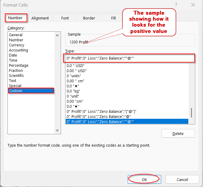
➤ In the Type box, write the following conditional suffix-
0″ Profit”;0″ Loss”;”Zero Balance”;””@””
This condition refers to 0 “Profit displays Profit after positive value, 0 “ Loss” after negative value, and “Zero Balance” in the place of 0. The ““@”” gives the text value as it is.
➤ Click OK.
➤ After formatting, the data table will be added with the conditional suffixes.
Notes:
You can also color-code them along with the texts for different values. For example, if you want green colored text for profit and red colored text for loss, use this in the Type box-
[Green]0″ Profit”;[Red]0″ Loss”;”Zero Balance”;””@””
Scale Numbers to Add Thousands/Millions as Suffixes
In large datasets, not only do we need to deal with large amounts of data, but our numbers also become larger. In financial documents, population data, and sales summaries, this becomes quite hard to read. Of course, 25,000,000 seems less intuitive than 25M (million). The good thing is you can also use Excel’s Custom Format option to add units of thousands (K), millions (M), billions (B), or even as per your requirements.
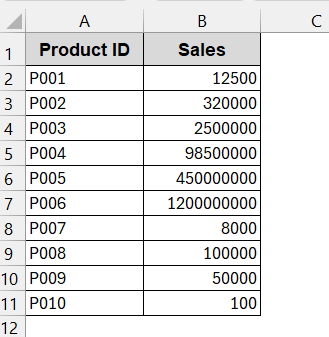
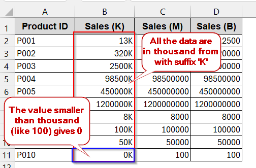
For the sake of this method, we will use this example of the dataset. Here we will convert the Sales into thousands. Millions and billions, creating three different columns for each.
Steps:
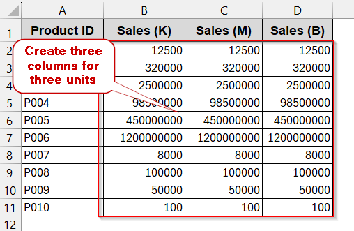
➤ Open the dataset, and create another two columns for sales, copying the first column.
➤ Give a proper header mentioning the units.
➤ Select column B (Sales (K)), and press Ctrl + 1 .
➤ In the Format Cells window, go to the Number tab and choose Custom from Category.
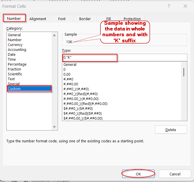
➤ In the Type section, write the following for the thousand unit by using K–
0,”K”,
Here, zero ensures the values are in whole numbers.
➤ Click OK to apply.
➤ Now, select column C (Sales (M)), and go to the Format Cells window again.
➤ In the Type box, now write –
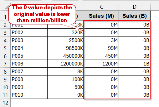
0,,”M”
➤ For the third column of Sales (B), follow the same steps and in the Type box, enter-
0,,,”B”
Notes:
The comma means the original value is divided by 1000. For two or more commas, the value is divided by 1000 twice or more times.
Custom Format Special Characters and Symbols after Number
We are not always going to add texts or units to the dataset. We may also need to add symbols after our raw numbers to make sense of them. Just like, we need to add degrees Celsius (°C) after temperature values and so on. As Excel does not have a pre-built formatting for such a situation, we have to opt for the Custom Formatting option again.
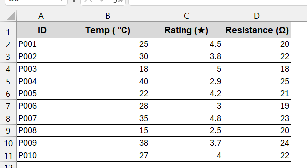
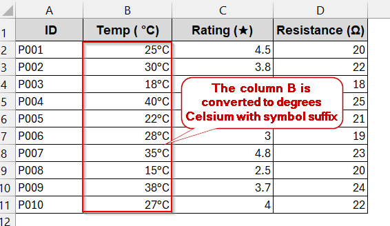
For special cases, we will be using the dataset below. It contains values of Temp (°C), Rating (★), and Resistance (Ω).
Steps:
➤ Open the dataset and determine the symbols required.
➤ Select the column of Temp (°C) and open the Format Cells window.
➤ Go to the Number tab and choose Custom from Category.
➤ In the Type box, type –
0″°C”
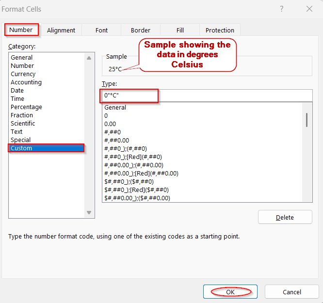
➤ Click OK to confirm.
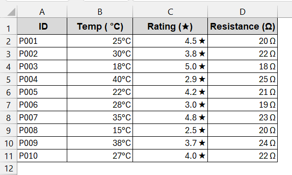
➤ Follow the same process of the Ratings(★) column and in the Type box of the Format Cells window, enter –
0.0″ ★”
➤ For the Resistance (Ω) column, write the below formatting in the Type box –
0″ Ω”
➤ Finally, all the columns are formatted with the customized symbols.
Notes:
These symbols are not part of the Excel built-in formats. It is best to copy and paste them when applying them to the Type box.
VBA Macro Alternatives for Custom Formatting
The custom formats are effective until you export or share your datasets. The Custom Format in the Format Cells option does not work; it just shows plain numbers. For advanced use cases like this, VBA Macros help you format the cells with texts and numbers permanently if you save your workbook as macro-enabled (.xlsm). The outputs are permanent text strings and are self-explanatory.
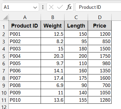
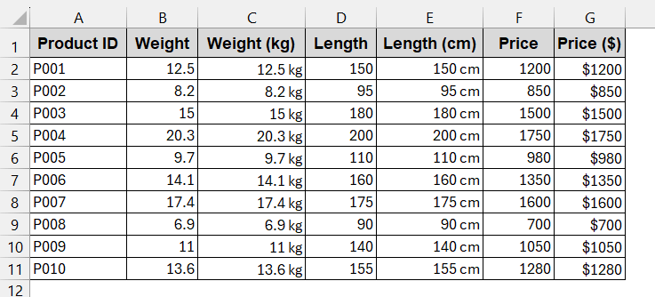
A basic dataset with columns for Weight, Length, and Price is used for this method.
Steps:
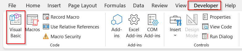
➤ Open the dataset, go to the Developer tab, and click Visual Basic.
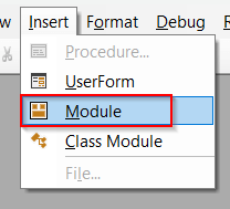
➤ In the Visual Basic window, click the Insert tab and choose Module.
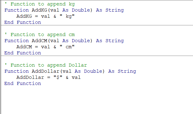
➤ Paste the following code in the space –
' Function to append kg
Function AddKG(val As Double) As String
    AddKG = val & " kg"
End Function
' Function to append cm
Function AddCM(val As Double) As String
    AddCM = val & " cm"
End Function
' Function to append Dollar
Function AddDollar(val As Double) As String
    AddDollar = "$" & val
End Function
➤ Save the VBA code and close the window.
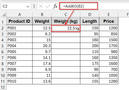
➤ Create a new column to store the weight in kg.
➤ In the first cell of the column, write the VBA formula –
=AddKG(B2)
where B2 is the cell with the weight of the previous column.
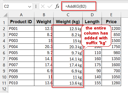
➤ Use Fill Handle to use the same formula for the rest of the cells.
➤ Add a new column for the Length and Price, respectively.
➤ Write the formula of the length function in the new length column –
=AddCM(C2)
➤ Write the formula of the price function in the new column –
=AddDollar(D2)
➤ Use Fill Handle to get the results in all of the cells.
Notes:
Unlike other methods, VBA Macros change the values in text and can’t be used in further calculations.
Frequently Asked Questions (FAQs)
How do I keep the number numeric after adding text?
You can keep the number numeric after adding text if you format the cells using Custom Format. Right-click to select the Format Cells option. In the window, choose the Category to Custom from the Number tab and add the text accordingly.
Can I add text only for positive numbers?
You can add text for only positive numbers by using conditions while formatting. In the Type box, you need to specify the condition as needed.
Will custom formats export with text to CSV?
The custom formats do not get exported with texts to CSV. It will only show the plain text. If you want to export or share the data, use the VBA method or the CONCAT formula to add text. It will change the number to a text string instead of a numeric one.
How to show currencies for different locales?
By default, Excel has the dollar ($) sign for currency formatting. To choose a different currency symbol based on locales, go to the Format Cells window. From the Number tab, select Currency as the category. In the Symbol box, click the arrow to choose a different currency for different locations.
How to quickly add a dollar sign ($) in Excel
The dollar sign ($) is available in the Format Cells window and does not require a Custom Format. You can directly select Currency or Accounting category to apply the formatting. Also, in the Home tab, under the Number section, you will find the shortcut for the Accounting ($) sign.
Concluding Words
Making your data meaningful in Excel does not always mean adding hefty formulas. Sometimes, a simple formatting can do the job with precision and style without breaking the data type. Whether your goal is to add units like kilogram and dollars, scalable numeric units for thousand, million, and billion, or special symbols, you can completely trust the Custom Format option of Excel. Along with handling all these options, it also gives you flexibility in adding different conditional texts for different numeric values. However, if you want to export your data, you can opt for VBA Macros, which are specially suited for bulk and permanent changes.
As you go through each method, you will discover that each method has its own uniqueness paired with its limitations. Follow the steps, use the strength of each, and apply it to your datasets to transform them into a more practical and professional workbook.