When working with multiple sheets in Excel, it’s common to want to fetch or display data from one sheet based on a value in another sheet. But many users struggle with setting this up correctly. Relying on manual copy-pasting or searching through sheets wastes time and increases the risk of errors. However, Excel provides efficient built-in functions and tools that can pull data dynamically from another sheet, based on a cell value. This makes your spreadsheets more interactive, automated, and easier to maintain.
In this article, we’ll learn several effective methods to get data from another sheet based on a cell value using functions like INDIRECT, VLOOKUP, HLOOKUP, INDEX and Advanced filter tool. Let’s get started.
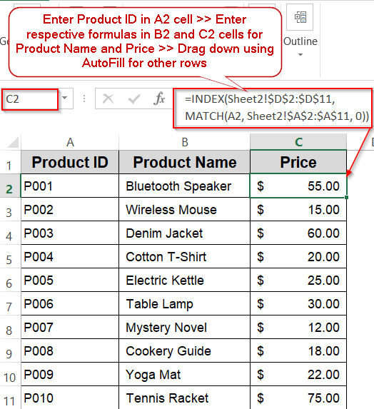
Steps to get data from another sheet based on cell value in Excel:
➤ Suppose in Sheet1, you enter a Product ID in cell A2 (P001 for example).
➤ To get the Product Name in B2, enter this formula:
=INDEX(Sheet2!$C$2:$C$11, MATCH(A2, Sheet2!$A$2:$A$11, 0))
➤ To get the Price in C2, enter this formula:
=INDEX(Sheet2!$D$2:$D$11, MATCH(A2, Sheet2!$A$2:$A$11, 0))
➤ Drag the formula down to apply for other rows.
Insert INDEX and MATCH Functions to Retrieve Data From Another Sheet
The combination of INDEX and MATCH is one of the most efficient ways to look up data based on a criteria in Excel which allows you to search in any direction (left or right), is not affected by column insertions, and works faster for large datasets. In this approach, the MATCH function searches for the position of your lookup value in the source range, and the INDEX function returns the corresponding value from another column based on that position.
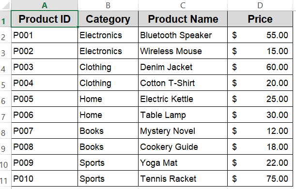
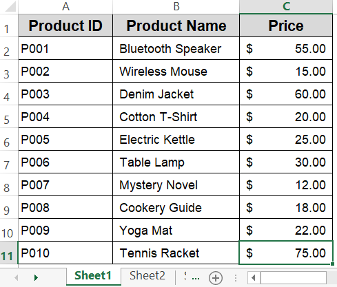
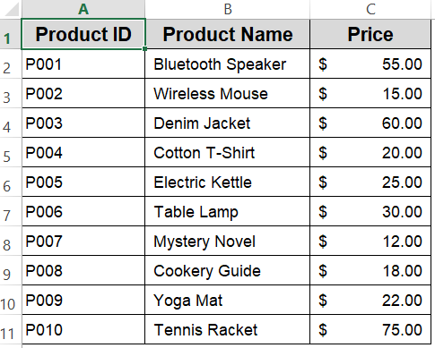
We will retrieve data from a sheet called Sheet2 containing details about different products. Our goal is to find information like Product Name and Price just by typing the relevant Product ID in another sheet.
Steps:
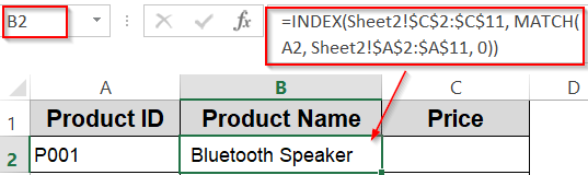
➤ Suppose in Sheet1, you enter a Product ID in cell A2 (P001 for example).
➤ To get the Product Name in B2, enter this formula:
=INDEX(Sheet2!$C$2:$C$11, MATCH(A2, Sheet2!$A$2:$A$11, 0))
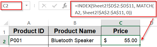
➤ To get the Price in C2, enter this formula:
=INDEX(Sheet2!$D$2:$D$11, MATCH(A2, Sheet2!$A$2:$A$11, 0))
➤ Drag the formula down to apply for other rows.
This formula dynamically pulls the Category and Price from Sheet2 based on the Product ID typed in Sheet1.
Use VLOOKUP Function to Fetch Data From Another Sheet
VLOOKUP is one of the most popular and easy-to-use lookup functions in Excel, widely used for finding information in structured tables. It searches for a given value in the leftmost column of a specified range and returns the corresponding value from a column to the right. The main advantage of the VLOOKUP function is its simplicity and quick setup, making it ideal for beginners and for datasets where the structure is fixed.
We’ll use the VLOOKUP function to find information like Product Name and Price just by typing the relevant Product ID in another sheet.
Steps:
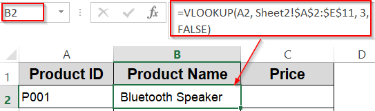
➤ In another sheet, type a Product ID in cell A2 such as P001.
➤ Enter this formula in B2 to get Product Name:
=VLOOKUP(A2, Sheet2!$A$2:$E$11, 3, FALSE)
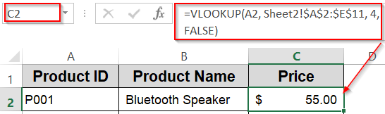
➤ To get the Price in C2, enter this formula:
=VLOOKUP(A2, Sheet2!$A$2:$E$11, 4, FALSE)
➤ Copy the formula down to apply to other rows.
This method is straightforward but requires that the lookup column be the first column in the source range.
Dynamically Reference Specific Cell from Another Sheet with INDIRECT Function
When working with multiple sheets or large datasets, constantly editing formulas to point to different locations can be tedious. The INDIRECT function solves this by turning text into an actual reference, letting you control both the sheet name and the cell address from other cells. This is especially useful when building dashboards or summary sheets that pull information from a master dataset like your product list in Sheet2 without changing the formula itself.
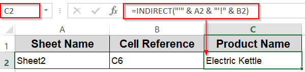
For example, you could type Sheet2 in one cell and C6 in another, and the formula will instantly return Electric Kettle from your dataset. Change the sheet name to point to another source, or adjust the cell reference to fetch a different product detail such as the price, and the results update automatically.
Steps:
➤ In a new sheet, type the sheet name Sheet2 in A2.
➤ In B2, type the cell reference you want to fetch, e.g., C6 (which holds Electric Kettle in Sheet2).
➤ Enter this formula in C2:
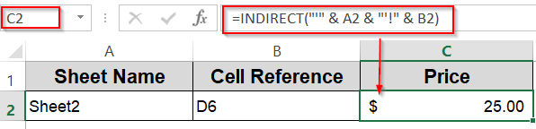
=INDIRECT("'" & A2 & "'!" & B2)
➤ Electric Kettle will display immediately from Sheet2.
➤ Change A2 to another sheet name or B2 to another cell reference (e.g., D6 for the price $25.00), and the output updates instantly.
Retrieve Data from a Horizontal Layout with HLOOKUP Function
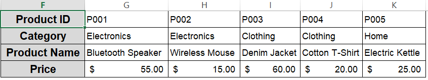
If your dataset is arranged horizontally with Product IDs running across the first row and related details in rows beneath, HLOOKUP function is the go-to function. It scans the top row from left to right, finds your lookup value, and returns the matching data from the row you specify. For example, if P004 is in the first row and prices are stored in the third row, HLOOKUP can instantly return $20.00 without manual searching.
Steps:
➤ In Sheet2, arrange your dataset horizontally with Product IDs in G1:K1, Categories in the 2nd row, Product Names in the 3rd row, and Prices in the 4th row.
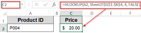
➤ In Sheet1, enter the lookup Product ID in A2 (e.g., P004).
➤ Enter this formula in C2 cell:
=HLOOKUP(A2, Sheet2!$G$1:$K$4, 4, FALSE)
➤ This returns the price for the given Product ID such as P004, it will return $20.00.
Note:
Our original dataset in Sheet2 is vertical, so you’d need to transpose it to test HLOOKUP directly.
Filter Matching Rows from Another Sheet with Advanced Filter
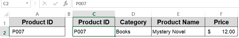
If you need to pull a full row of details from another sheet, not just a single value, then the Advanced Filter feature can do it quickly. It copies matching records to a new location while leaving your source data untouched. For example, entering P007 as a Product ID in Sheet1 can instantly bring over the full record such as Product ID, Name, Category and Price from Sheet2.
Steps:
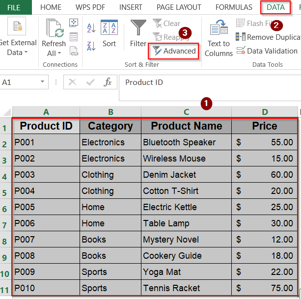
➤ In Sheet2, select your dataset A1:D11.
➤ Go to the Data tab >> Advanced (in the Sort & Filter group).
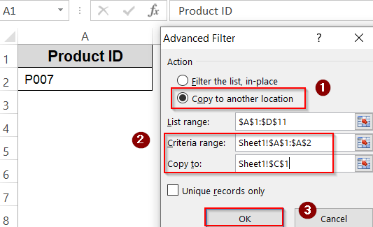
➤ In the Advanced Filter dialog, choose Copy to another location.
➤ Set Criteria range to Sheet1!A1:A2 (A1 = “Product ID“, A2 = your search ID like P007).
➤ Set Copy to a blank cell in Sheet1 (e.g., C1).
➤ Click OK and the full matching row from Sheet2 will be copied.
This method is great for filtering multiple matching rows or complex criteria.
Frequently Asked Questions
Can I use these methods if my data is in different workbooks?
Yes. You can use all these formulas across multiple workbooks. Just ensure the source workbook is open or properly linked. If the source file is closed, some functions may slow down or return errors unless external references are properly established.
What if my lookup value is not found?
When the lookup value doesn’t exist in the source data, formulas like VLOOKUP or INDEX/MATCH will return an error. To avoid this, wrap your formulas with IFERROR function to display a custom message such as “Not Found” or leave the cell blank gracefully.
Which method is best for large datasets?
For large datasets, the combination of INDEX and MATCH functions tend to be more efficient and faster than VLOOKUP function, which can slow down spreadsheets. However, INDIRECT function is volatile and recalculates frequently, potentially reducing performance in big workbooks.
Can I retrieve multiple columns at once?
Yes, you can retrieve data from multiple columns by extending your INDEX ranges or using multiple VLOOKUP formulas for each column. If you have Excel 365 or 2021, the XLOOKUP function simplifies this by returning multiple columns with a single formula.
Wrapping Up
In this tutorial, we’ve learned how to efficiently get data from another sheet in Excel based on a cell value using five different methods. From the classic VLOOKUP to the more flexible INDEX and MATCH functions, and even dynamic references with INDIRECT function or filtering with Advanced Filter, each method has unique strengths. Understanding these techniques helps you to create dynamic and automated spreadsheets that save time and reduce errors. Feel free to download the practice file and share your feedback.