
When you are working with large data tables in Excel, you often need to search for values both vertically and horizontally. Neither lookup function is flexible when column or row positions change. When you want to find a value that lies at the intersection of a column and a row, you need to combine VLOOKUP and HLOOKUP. Combining VLOOKUP and HLOOKUP functions will help you perform powerful lookups in complex datasets. In this article, you’ll learn different ways to combine VLOOKUP and HLOOKUP in Excel
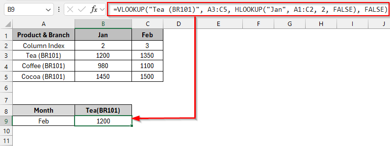
To find the January sale of the Tea(BR101) product, you can use the HLOOKUP function inside the VLOOKUP function.
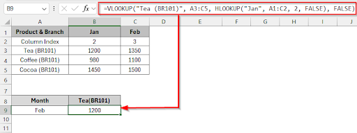
➤ Select the cell B9 and write this formula:=VLOOKUP(“Tea (BR101)”, A3:C5, HLOOKUP(“Jan”, A1:C2, 2, FALSE), FALSE)
➤ Press Enter and see the result of the January sale of the Tea(BR101) product, which is 1200.
This article explores four methods for combining VLOOKUP and HLOOKUP in Excel. Combine VLOOKUP with MATCH function, Combine HLOOKUP with MATCH function, Using the HLOOKUP inside the VLOOKUP function, using XLOOKUP for Both Row & Column Lookup are the four methods to combine VLOOKUP and HLOOKUP in Excel.
Short Overview of the VLOOKUP and HLOOKUP Functions in Excel
VLOOKUP: VLOOKUP means vertical lookup. It is the lookup function to search for a value in the first column of a table and return a value from the same row.
VLOOKUP function syntax: VLOOKUP(lookup_value, table_array, col_index_num, [range_lookup])
HLOOKUP: HLOOKUP means horizontal lookup. It is the lookup function to search for a value in the first row of a table and return a value from the same column.
HLOOKUP function syntax: HLOOKUP(lookup_value, table_array, row_index_num, [range_lookup])
Example with VLOOKUP Function
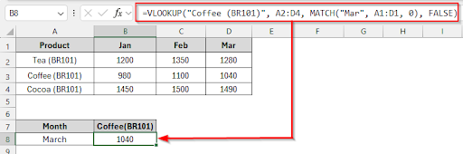
The VLOOKUP function is used to search values vertically in a table with a fixed column number to return results. Using the MATCH function with the VLOOKUP function helps to find that column number automatically.
Let’s look at the dataset below, where we want to find the March month sale value of the coffee(BR101) product, combining the VLOOKUP with the MATCH function.
Steps:
➤ Click on the cell B8 and write this formula:
=VLOOKUP("Coffee (BR101)", A2:D4, MATCH("Mar", A1:D1, 0), FALSE)
➤ Press Enter and see the result. The march month value of coffee(BR101) is 1040
Example with the HLOOKUP Function
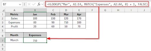
The HLOOKUP function searches horizontally across the top row of a table. By combining HLOOKUP with the MATCH function, you can find the correct row number based on a lookup value.
Let’s look at the dataset below, where the dataset is about sales, expenses and profit of Jan, Feb, Mar, and April. We will find the March expenses, and the result will be in the B7 cell.
Steps:
➤ Click on the cell B7 and write this formula:
=HLOOKUP("Mar", A1:E4, MATCH("Expenses", A2:A4, 0) + 1, FALSE)
➤ Press Enter and see the result. The March expenses value is 710
Combining HLOOKUP with the VLOOKUP Function
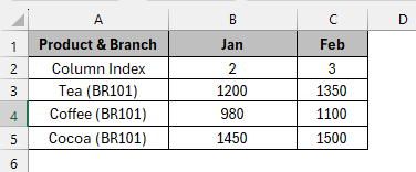
The HLOOKUP function within VLOOKUP is a nested formula, which is useful for dynamically selecting the correct column number based on the month name. You don’t need to count the column index manually. From a helper row, the HLOOKUP function will return the column number.
In this method, we will find the January sale of the Tea(BR101) product in cell E3. We will use the HLOOKUP function inside the VLOOKUP function to find the value.
➤ Select the cell B9 and write this formula:
=VLOOKUP("Tea (BR101)", A3:C5, HLOOKUP("Jan", A1:C2, 2, FALSE), FALSE)
➤ Press Enter and see the result of the January sale of the Tea(BR101) product, which is 1200.
Alternative to VLOOKUP-HLOOKUP Combined: XLOOKUP for Two-Way Lookup
The XLOOKUP function can look up both rows and columns easily and replaces both the VLOOKUP and HLOOKUP functions.
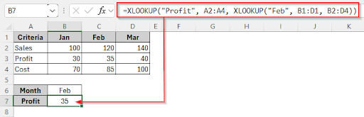
This is the most suitable method for 2D lookup. Here, we will use the double or nested XLOOKUP. The Inner XLOOKUP gets the column & the outer XLOOKUP gets the row from that column.
Steps:
➤ Click on cell B7, and write the formula:
=XLOOKUP("Profit", A2:A4, XLOOKUP("Feb", B1:D1, B2:D4))
➤ Press Enter and see the result of the February profit, which is 35.
Frequently Asked Questions
If the lookup value is not found, what will be the result?
The VLOOKUP and HLOOKUP formulas will return a #N/A error if the lookup values do not find an exact match.
How can we use the MATCH function instead of combining the VLOOKUP and HLOOKUP functions?
Using the MATCH function helps to find that column number automatically. The formula will be:
=INDEX(B3:E11, MATCH(“Cocoa (BR202)”, A3:A11, 0), MATCH(“Apr”, B1:E1, 0))
What are the reasons to get a #VALUE! error when combining VLOOKUP and HLOOKUP?
The reason to get a #VALUE! error if the column or row index is not a valid number
If HLOOKUP or VLOOKUP references the wrong range (e.g., headers not included properly), the lookup value is spelt incorrectly or not found, or if the helper row or column is missing.
What are the reasons to get a #N/A error while using the VLOOKUP or HLOOKUP function?
You can get a #N/A error if the lookup value doesn’t exist in the lookup range, the range is incorrect, or not properly locked ($A$1:$C$10), the match type is wrong (e.g., using TRUE for an approximate match instead of FALSE for an exact), there’s a mismatch in data format (e.g., text vs number).
Wrapping Up
You can handle more complex and dynamic datasets in Excel by combining VLOOKUP and HLOOKUP functions. In this article, we explored four different ways to combine VLOOKUP and HLOOKUP in Excel. We have discussed combining VLOOKUP with MATCH function, combining HLOOKUP with MATCH Function, HLOOKUP inside VLOOKUP function, XLOOKUP function for Both Row and Column functions. Feel free to download the practice file and share your thoughts and suggestions.