Random or unbiased selection from a list of names, numbers, or dates is useful for surveys, data analysis, market research, etc. Excel doesn’t have any built-in feature or direct formula to select one or multiple values from a list.
Therefore, we need to combine several functions to randomize a list.
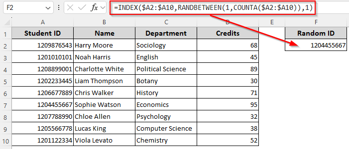
The most effective approach to randomly choose one or more cells from a list is to combine the INDEX, RANDBETWEEN, and COUNTA functions.
Steps to select random values using the INDEX, RANDBETWEEN, and COUNTA functions:
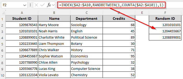
➤ Select a cell where you want to put the first random value and insert the following formula:
=INDEX($A2:$A10,RANDBETWEEN(1,COUNTA($A2:$A10)),1)
➤ Here, $A1:$A10 is the range from which we’ll select randomly. Change the range as needed.
➤ Press Enter and Excel will return a random value from your selected range. If you want more values, drag the formula down to as many cells you want.
While this formula works, it might return duplicate values. Whether you want to select randomly with formulas, manual steps, or with/without duplicates, this article covers all the ways including using the data analysis toolbar, sorting, VBA coding, and functions like INDEX, RAND, RANDBETWEEN, RANK, etc.
Manually Select Random Values with the Data Analysis Feature
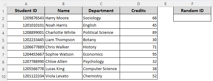
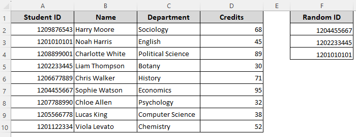
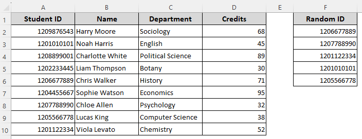
In our dataset, we have columns for student IDs, names, department, and other details. Our goal is to select one or multiple IDs randomly from column A. We’ll put the randomly selected data in column F.
In the Data Analysis Toolbar, you can use the Sampling option and select one or more numeric values (such as phone numbers and IDS) randomly in a selected output range. Keep in mind that this method only works for numeric values. Here are the steps:
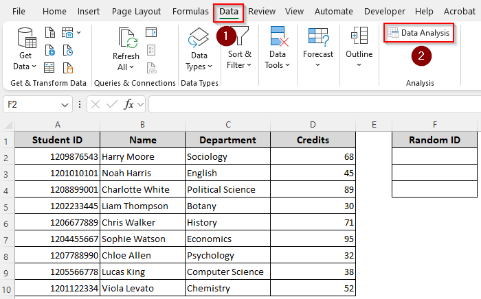
➤ Click on the Data tab and select Data Analysis from the Analysis group.
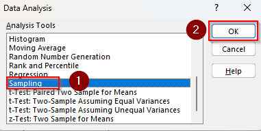
➤ As the Data Analysis dialog box opens, scroll down and select Sampling from the Analysis Tools options. Press Ok.
➤ Now, a new Sampling window will open. In the Input Range box, manually type or highlight the input range from where you want to select randomly.
➤ From the Sampling Method group, select Random and enter a number in the Number of Samples box to define how many random samples you want to extract.
➤ In the Output options, choose Output Range and manually type or highlight the cells to put the extracted random samples.
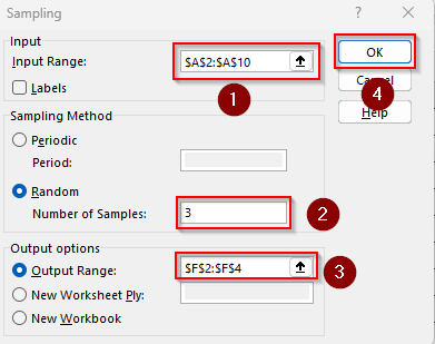
➤ Finally, click Ok and Excel will return the random values.
Return Random Values Based on Different Criteria
In Excel, the COUNTA function counts the number of non-blank cells in a range. While the RANDBETWEEN function assigns one random number from your specified range, the INDEX function returns one value from the range, based on that random number.
However, as you drag the formula down, it might return duplicate values. Here’s how to combine them to pick only one random value:
➤ Choose a cell where you want to put the first random value and enter any of the following formulas:
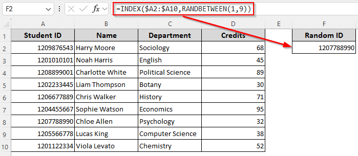
For a Fixed Number of Rows
If you know how many rows consist the list, insert the following formula:
=INDEX($A2:$A10,RANDBETWEEN(1,9))
➤ Replace the list range $A2:$A10 and number of rows according to your dataset. Click Ok.
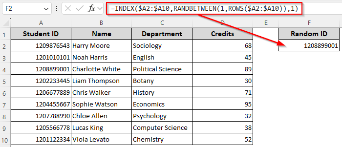
For a List with Non-Blank Cells
Use the following formula if you don’t know the number of rows and your list doesn’t have any blank cells:
=INDEX($A2:$A10,RANDBETWEEN(1,ROWS($A2:$A10)),1)
➤ Change the list range as required and press Enter.
For a List with Blank and Non-Blank Cells
When you don’t know the number of rows and the cells are a mix of blank and non-blank cells, use the formula given below:
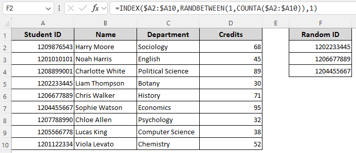
=INDEX($A2:$A10,RANDBETWEEN(1,COUNTA($A2:$A10)),1)
➤ Replace the list range if needed and press Ok.
➤ If you want more than one random value, you can drag the formula down using the fill handle (+ sign on the bottom corner of the cell).
Dynamic Array Sampling of Random Values from the List
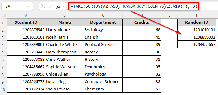
If you use Excel 365, the easiest way to select randomly is by applying the TAKE, SORTBY, RANDARRAY, and COUNTA functions. First, the COUNTA function counts the number of non-empty cells in a range. After that, the RANDARRAY function generates an array of random numbers for those cells.
While the SORTBY function sorts the array based on the values in one or more corresponding arrays, the TAKE function returns a specified number of rows or columns from the start or end of an array. Here’s how to use them in a formula to return random values without duplicates:
➤ In a cell where you want to first random value, insert the following formula:
=TAKE(SORTBY(A2:A10, RANDARRAY(COUNTA(A2:A10))), 3)
➤ This formula returns 3 random IDs from column A. Change the list range A2:A10 and number of returned values 3 according to your dataset.
➤ Press Enter.
Random Selection with RAND Function
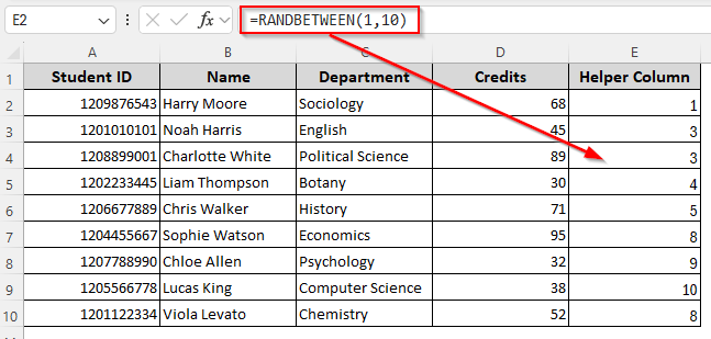
With the RAND function, you can assign random numbers to each row of your selection. The RANDBETWEEN function does the same, except that it only assigns integers instead of fractions. While using this method, we’ll assign a random number to each row. After that, we’ll apply a formula to extract random values in a different location.
For this, we’ll use the RANK function to return the rank of a number within a list. Later on, the INDEX function will return the value for that specific position. Let’s get to the process:
➤ In a helper column cell, insert any of the following formulas:
=RAND()
Or,
=RANDBETWEEN(1,10)
➤ Replace the number of rows as necessary. Click Enter and drag the formula down.
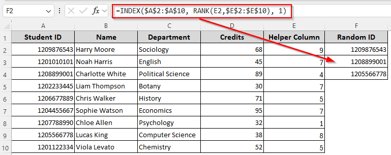
➤ Now, in a different cell (cell F2) where you want to put the first random value, enter this formula:
=INDEX($A$2:$A$10, RANK(E2,$E$2:$E$10), 1)
➤ Here, A$2:$A$10 is the range from where you’re choosing randomly. E2 is the first cell of the helper column and $E$2:$E$10 is the entire helper column range. Change the values as needed.
➤ Now, Excel will return the first randomly selected value. You can drag the formula down to get more.
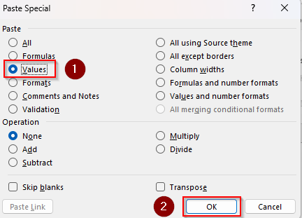
➤ If you want to delete the helper column, copy the output values with the CTRL + C shortcut. Now, right-click on the same values and select Paste Special >> Values >> Ok.
Customize VBA Macro to Randomly Select from a List
For larger datasets, it’s better to use a custom VBA specifically coded to return random values. It allows you to choose as many values you want. Here’s how:
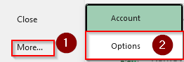
➤ To add the Developer tab in the top ribbon, go to Files >> More >> Options.
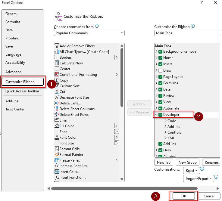
➤ Now, choose Customize Ribbon and click on the Developer box. Press Ok.
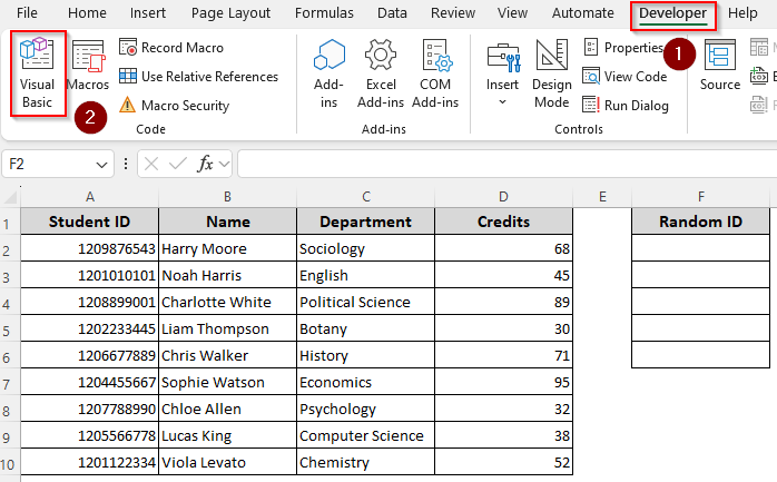
➤ Open the Developer tab from the top ribbon and select the Visual Basic option.
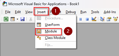
➤ In the VBA Editor, click on Insert and choose Module.
➤ Paste the following code in the module box:
Sub PickRandomValues()
Dim rngInput As Range
Dim rngOutputStart As Range
Dim inputValues() As Variant
Dim outputCount As Long
Dim pickedIndexes As Collection
Dim i As Long, index As Long
' Ask user to select the input range
On Error Resume Next
Set rngInput = Application.InputBox("Select the range of values to pick from:", "Input Range", Type:=8)
On Error GoTo 0
If rngInput Is Nothing Then Exit Sub
' Ask user how many values to pick
outputCount = Application.InputBox("How many random values do you want to pick?", "Number of Values", Type:=1)
If outputCount <= 0 Then Exit Sub
' Validate the number of picks
If outputCount > rngInput.Cells.Count Then
MsgBox "You cannot pick more values than available in the list.", vbExclamation
Exit Sub
End If
' Ask user where to output the results
On Error Resume Next
Set rngOutputStart = Application.InputBox("Select the first cell for output:", "Output Cell", Type:=8)
On Error GoTo 0
If rngOutputStart Is Nothing Then Exit Sub
' Store values in array
inputValues = rngInput.Value
' Initialize collection to store unique random indexes
Set pickedIndexes = New Collection
Randomize
Do While pickedIndexes.Count < outputCount
index = Int((rngInput.Cells.Count) ➤ Rnd + 1)
On Error Resume Next
pickedIndexes.Add index, CStr(index)
On Error GoTo 0
Loop
' Output selected values
For i = 1 To pickedIndexes.Count
rngOutputStart.Cells(i, 1).Value = rngInput.Cells(pickedIndexes(i), 1).Value
Next i
MsgBox outputCount & " random value(s) picked successfully!", vbInformation
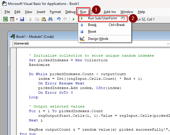
End Sub➤ Click on the Run tab >> Run Sub/UserForm. You can also press F5 instead.
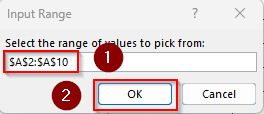
➤ As Excel prompts you, go back to the Excel tab and select the input cell range or list from where you want to choose random values. Click Ok.
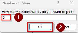
➤ Now, in the Number of Values box, define how many random values you want and press Ok.
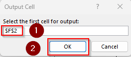
➤ Finally, choose an output cell for the returned value(s) selected randomly.
➤ As you click Ok, Excel will show the result like this:
Frequently Asked Questions
How to randomly select cells based on criteria in Excel?
Let’s say we’re selecting 3 random employees from the Sales department. To select randomly based on this criteria, enter the following formula in a blank cell:
=INDEX(A:A, AGGREGATE(15,6,ROW(A2:A10)/(B2:B10=”Sales”), RANDBETWEEN(1,COUNTIF(B2:B10,”Sales”))))
If the criteria Sales is found in the range B2:B10, Excel will randomly return a value from the corresponding cells of column A (A2:A10 range).
How to randomly group a list in Excel?
If we have 20 names in A2:A21 and we want to make 4 random groups, first, we’ll create a helper column (column B) and enter this formula:
=RAND()
Press Enter and drag down. Now, select your entire data range and sort them by the helper column (smallest to largest). Finally, use a different column (column C) to assign groups using this formula:
=MOD(ROW()-2, 4)+1
As you press Enter and drag down, this formula gives group numbers 1 to 4 repeatedly.
How to rank randomly in Excel?
Create a helper column (column B) and insert this formula:
=RAND()
Click Enter and drag down. In a new column (column C), enter this formula:
=RANK.EQ(B2, $B$2:$B$10, 1)
It ranks all random numbers.
Concluding Words
As explained, there are several ways to select randomly from a list in Excel. Choose one based on your Excel version and your dataset’s requirements. However, keep in mind that all random functions recalculate with every worksheet change. If you want to freeze the results, copy them and use Paste Special >> Values.