How to Remove Last 3 Characters in Excel (4 Easy Methods)

In many Excel workflows you often need to remove a fixed number of trailing characters. It can be in time of cleaning up product codes, trimming status tags, or standardizing IDs. Removing the last three characters from each cell can help you group, sort, or analyze your data more effectively. There are several methods that we can use to remove the last 3 characters from a cell. We can even extend these methods to remove any number of characters when needed.

The LEFT & LEN functions can remove a fixed number of characters from a cell value. We will use that to remove the last 3 characters. Although it can remove any number of characters. The LEN function computes the string’s total length, and LEFT extracts the leftmost portion.

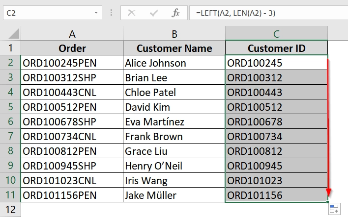
Here we have a dataset containing order details and customer name in two columns. However we want to keep the customer ID only by removing the last 3 characters from the order details.

Steps:

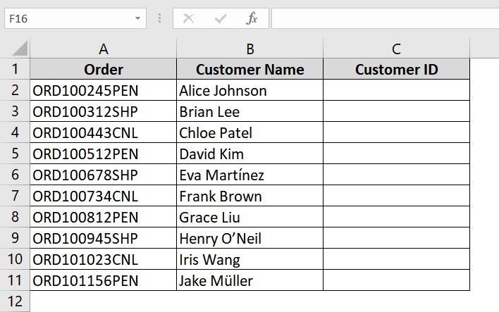
➤ Open up your dataset or use our dataset to practice. We have Order and Customer Name in the first two columns. We have named the third column as Customer ID to store the result after removing the last 3 characters from the Order details.

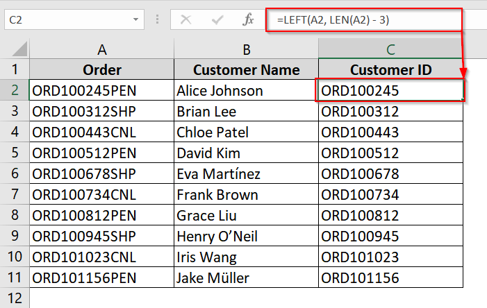
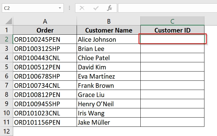
➤ Select the cell where you want the truncated result. Here we have selected cell C2.

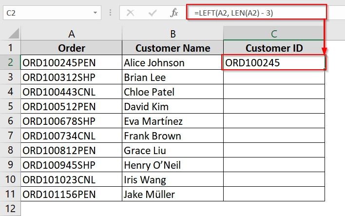
➤ Type the following formula and click Enter:

You should see the Customer ID in C2 (e.g., ORD100245).

➤ Now click the fill‑handle (the small square at the bottom‑right of C2) and drag down through C11 to apply the formula to all rows.

The REPLACE function can substitute a specified portion of text with an empty string. We will use this to replace the last three characters with empty string and thus we can easily remove those last three characters. You can use this function to replace any number of characters.

Steps:

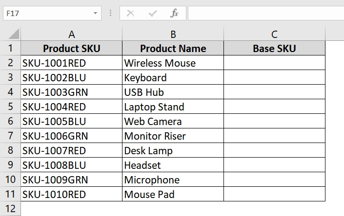
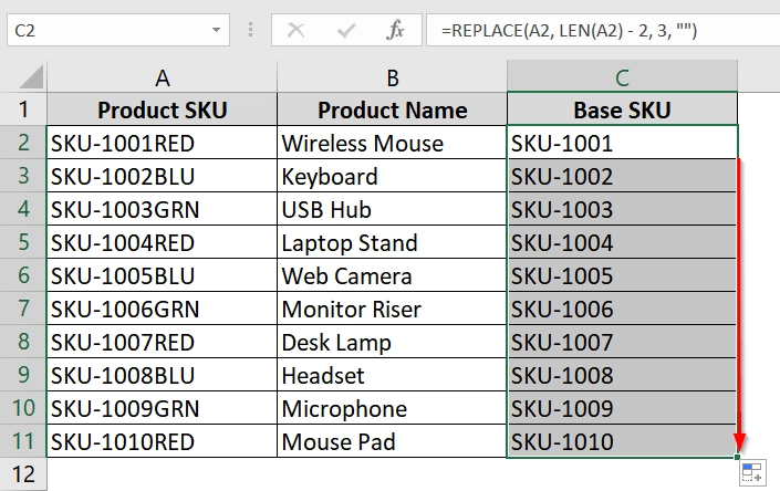
➤ Open up your excel dataset and follow the steps. Or you can use our dataset to practice. We have Product SKU in column A, Product Name in column B. We have named column C as Base SKU where we will store the result after replacing the last three character from column A.

➤ Click the cell C2,  type the formula and press Enter:

This tells Excel to start at the third‑from‑last character of A2 (LEN(A2)-2), remove 3 characters, and replace them with nothing. You will see the Base SKU in C2 (e.g., SKU-1001).

➤ Now drag the fill‑handle from C2 down to C11 to apply the formula to all rows.

Flash Fill is a built-in pattern recognition tool. It can automatically fill data based on the example you provide. It is best when your data follows a consistent pattern and you want a no‑formula approach.

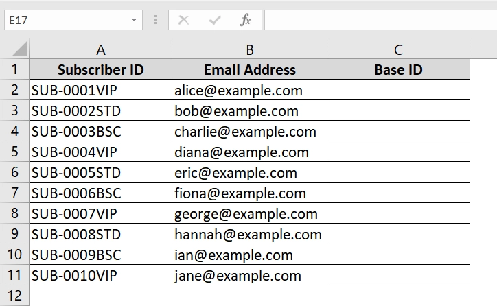
In our dataset we have Subscriber ID that has the same pattern consistency. So we can apply the Flash Fill method here.

Steps:

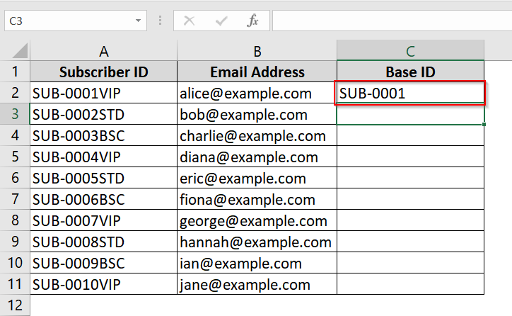
➤ Navigate to your dataset or download our provided dataset to practice. We have Subscriber ID in column A, Email Address in column B. We will remove the last three characters from the Subscriber ID and store them in column C. We have named column C as Base ID.

➤ In cell C2, enter SUB-0001 by manually removing -VIP and click Enter. We need to write this manually once so that excel can understand what pattern we want.

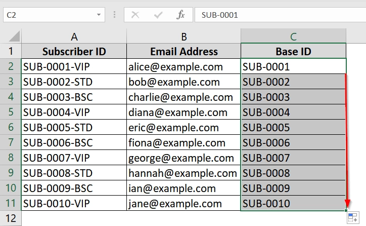
➤ Now drag the fill handle from the bottom right corner of the cell C2 from C2 to C11 to flash fill the rest of the cells. Excel will automatically detect the pattern and fill the rest of the cell accordingly.

We will create a VBA function that will remove the last three characters from a cell. e The advantage is we can highly customize these VBA functions  for our particular use cases and solve our tasks. We usually use this approach when we need a reusable function to remove any number of characters from the end of a string. It even works across multiple workbooks if modified accordingly.

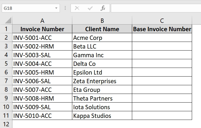
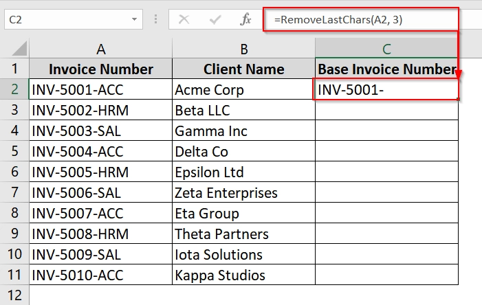
In our dataset we have Invoice Number in column A, Client Name in column B. We will remove the last three characters from Invoice number using a VBA function and store the result in column C. We have named column C as Base Invoice Number.

Steps:

➤ Open up your dataset.

➤ Press  Alt  +  F11  to launch the VBA Editor.

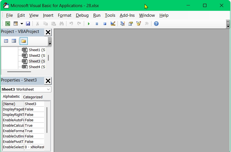
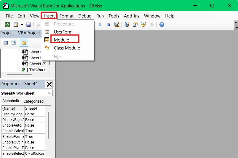
➤ In the VBA Editor, go to Insert > Module to add a new code module.

➤ In the code pane, paste the following function:

Function RemoveLastChars(str As String, num_chars As Long) As String
    If Len(str) > num_chars Then
        RemoveLastChars = Left(str, Len(str) - num_chars)
    Else
        RemoveLastChars = ""
    End If
End Function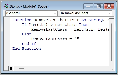

➤ Close the VBA Editor by clicking the X icon on top-right corner or pressing Alt + Q to return to Excel.
➤ In cell C2  enter the following formula and click Enter.

This calls your newly created function from VBA. It removes the last three characters of A2. The result looks like INV-5001-

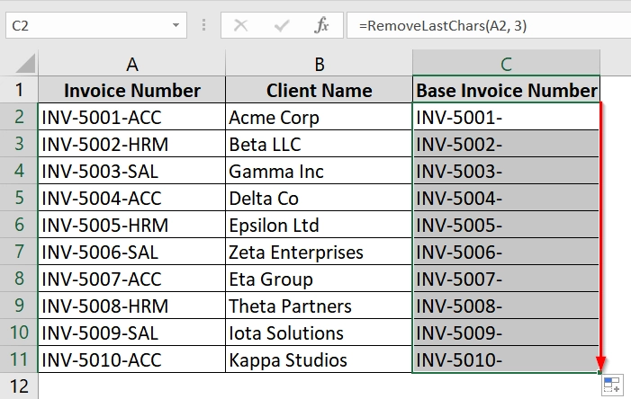
➤ Drag the fill‑handle from C2 down through C11 to apply the function to all other cell of the column.

Frequently Asked Questions (FAQs)

How do I remove the last 3 characters from an Excel cell?

Use the LEFT function combined with LEN: =LEFT(A1, LEN(A1)-3).

How do I remove the last 3 characters of a string?

In Excel, you can also use =REPLACE(A1, LEN(A1)-2, 3, “”) or Flash Fill for pattern‑based removal.

How do I delete 3 characters from the left in Excel?

Use the RIGHT function: =RIGHT(A1, LEN(A1)-3) to keep everything except the first three characters.

Concluding Words

We have discussed how to remove the last 3 characters from a cell value where we have shown 4 methods. The LEFT & LEN function is the most popular one. After that there is a REPLACE Function which replaces characters with empty strings. Then we have seen the Flash Fill method which is very easy to apply but only works if your data have a clear pattern. Lastly we have discussed how to deal with the VBA function. VBA functions are very useful and highly customizable.