When we are working with data in Excel we often need to import information from different sources like websites, CRMs, text files, or manual entries. These sources can add unwanted characters like extra spaces, special symbols, or fixed prefixes that disrupt our analysis or reporting. Excel has many easy to use methods that can easily remove these unwanted characters and make our dataset clean and ready for further operations.
To remove unwanted characters in Excel, follow these quick steps:
➤ Identify the type of unwanted character (e.g., extra space, prefix, or symbol).
➤ Use formula like =SUBSTITUTE(B2, “#”, “”) to remove unwanted characters.
➤ Replicate it down the column to apply the formula to other cells.
In this article, we will cover six Excel methods to remove unwanted characters. You will learn how to handle leading/trailing spaces, prefixes, special characters, or random noise using excel’s built in tools like Find and Replace, Flash Fill, function like LEFT, LEN, SUBSTITUTE, TRIM and others.
What Are Unwanted Characters in Excel?
Unwanted characters are any extra symbols, spaces, or text fragments that aren’t needed in your final data. These include:
- Spaces (leading, trailing, multiple)
- Special characters (like @, #, &, etc.)
- Prefixes or suffixes (like ID_, #2023)
- Random imported junk from uncleaned sources
Using Find & Replace Tool To Remove Unwanted Characters
The Find & Replace method is a simple way to remove specific unwanted characters from Excel data. You can use this method when you want to clean only one character at a time without affecting the rest of the content. It works best for feedback, notes, or comment columns where such symbols are unnecessary for analysis. However you can also remove multiple characters following the same process repeatedly .
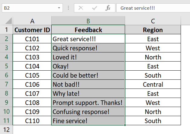
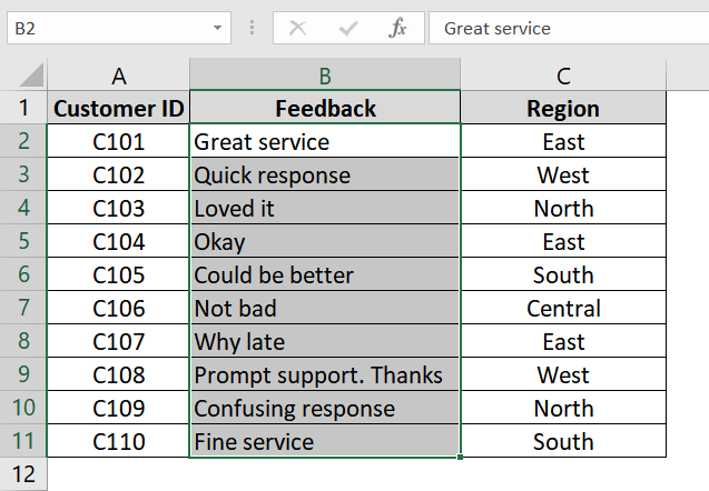
We have a dataset with customer feedback where only exclamation marks (!) need to be removed. These are not necessary for analysis and can affect data consistency or readability. We will use the Find & Replace tool to remove that exclamation mark character.
Steps:
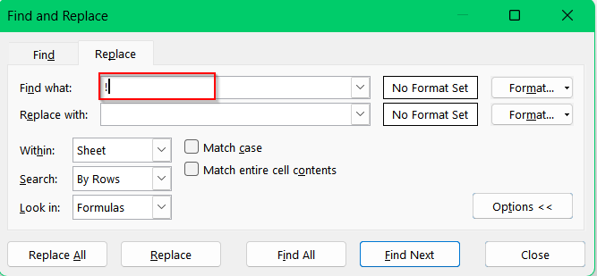
➤ Select the column that contains the exclamation marks. Click and drag to select the cells in your dataset (e.g., column B titled “Feedback”) where the text includes exclamation marks.
➤ Press Ctrl + H to bring up the Find and Replace dialog.
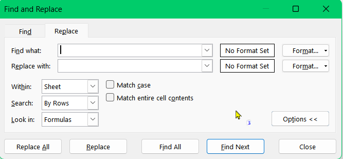
➤ In the “Find what:” box, type the exclamation mark (!) and leave the “Replace with:” box blank so Excel removes the character.
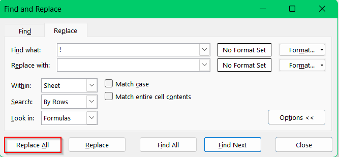
➤ Click “Replace All”
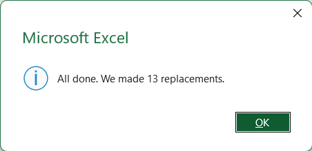
➤ A confirmation message will show how many replacements were made.
➤ Check the feedback column again and you will see that all exclamation marks have been removed properly.
Note:
If you only want to affect certain rows, highlight only those before running Find & Replace.
Applying SUBSTITUTE Function to Remove Unwanted Characters
The SUBSTITUTE function is used in Excel to replace specific unwanted characters within a cell. It is best used when the character you want to remove is consistent across the dataset and you need a formula-based approach instead of a manual one. This is helpful for cleaning up notes, comments, or names where characters like #, @, or ! etc have been mistakenly added.
Steps:
➤ Open your dataset. We have a dataset with Employee ID in column A, Comments in Column A and Department in Column C. The comments in Column B contains unwanted characters like “#”.
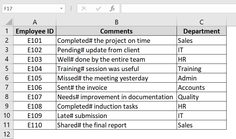
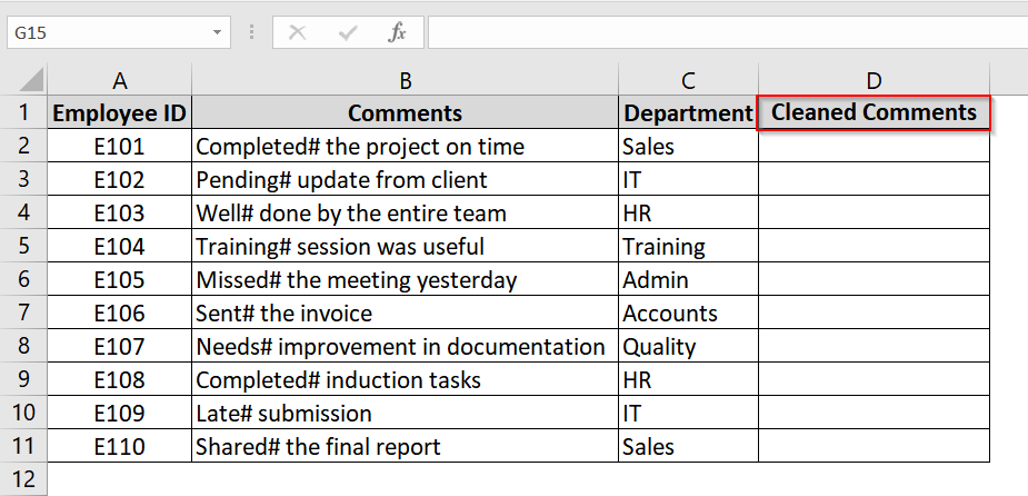
➤ Insert a new column (e.g., Column D) next to the comments column and title it “Cleaned Comments”.
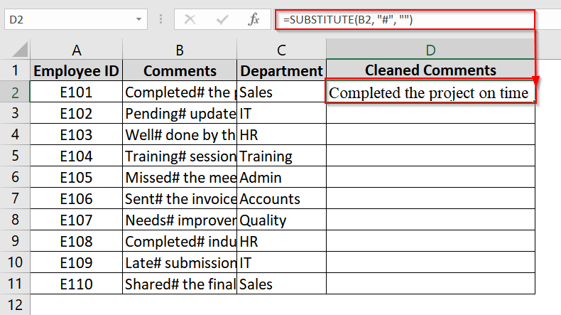
➤ In cell D2, enter the formula and click Enter:
=SUBSTITUTE(B2, “#”, “”)
This will remove the # symbol from the text in B2.
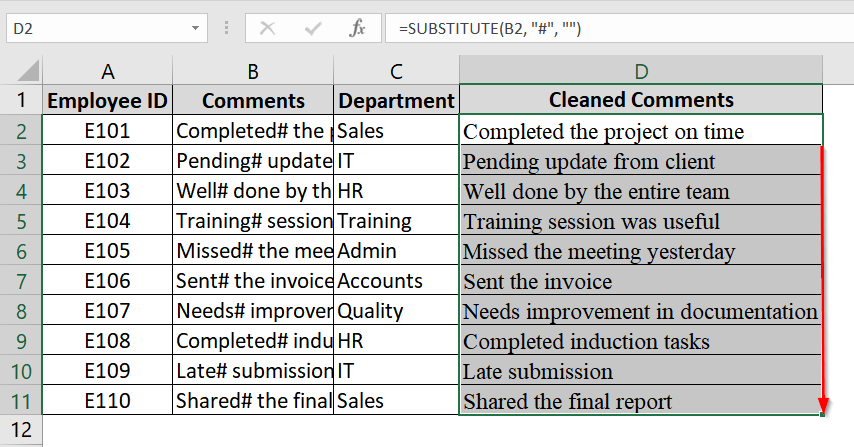
➤ Drag the fill handle from D2 down to D11 (or use Ctrl + D) to apply the formula to the rest of the rows.
Note:
➥ If you want to keep only the cleaned comments, you can copy Column D, then right-click on Column B and choose Paste Values to overwrite the old column.
➥ The SUBSTITUTE function is case-sensitive, but since we are removing symbols like #, it doesn’t matter.
➥ You can replace any specific character — like @, !, $, * — by changing the second argument in the formula.
Use TRIM Function to Remove Extra Spaces In Excel Dataset
The TRIM function in Excel is used to remove unnecessary spaces from text. It can delete all leading and trailing spaces and reduces any multiple spaces between words to a single space. This is very useful when we work with imported or manually entered data that contains inconsistent spacing in names, comments, or addresses.
Steps:
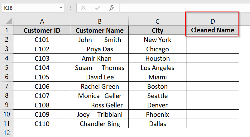
➤ Open your excel dataset. We have taken a dataset where we have the customer names in Column B, starting from B2 to B11, and contain extra spaces that need to be removed.

➤ Insert a new column next to Column B (e.g., Column D) and name it Cleaned Name.
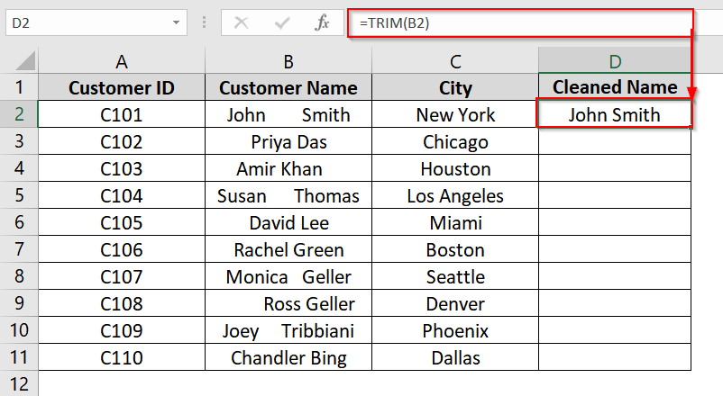
➤ In cell D2, enter the formula and click Enter:
=TRIM(B2)
This will remove all leading, trailing, and excessive in-between spaces from the text in cell B2.
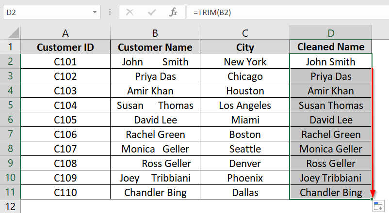
➤ Drag the fill handle from D2 down to D11 to apply the formula to the rest of the names.
Note:
➥ TRIM does not remove non-breaking spaces (imported from websites or databases). To handle those, use SUBSTITUTE together with TRIM.
➥ The function will not remove symbols or punctuation, it’s specifically for cleaning up space characters.
Using Flash Fill To Clean Any Type of Unwanted Characters
Flash Fill is an Excel feature that can automatically detect patterns based on user input and fill out data accordingly. We can use it for removing unwanted characters or text segments when there’s a recognizable pattern.
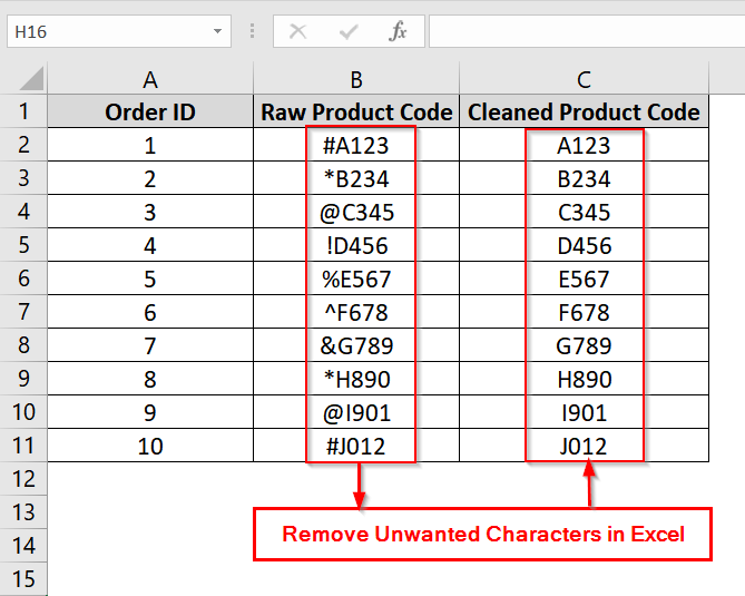
We have a dataset where we have product codes in Column B that contain unwanted special characters at the beginning (such as #, *, @). We will use Flash Fill so that Excel detects the pattern from the first manually entered clean value and auto-fills the rest without the unwanted symbols.
Steps:
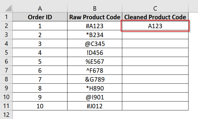
➤ Open up your dataset or use our example dataset. We have added a new column (e.g., Column C) and name it Cleaned Product Code.
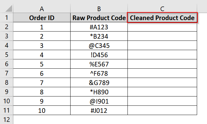
➤ In cell C2, type the cleaned version of B2. For example, enter A123 as B2 is #A123.
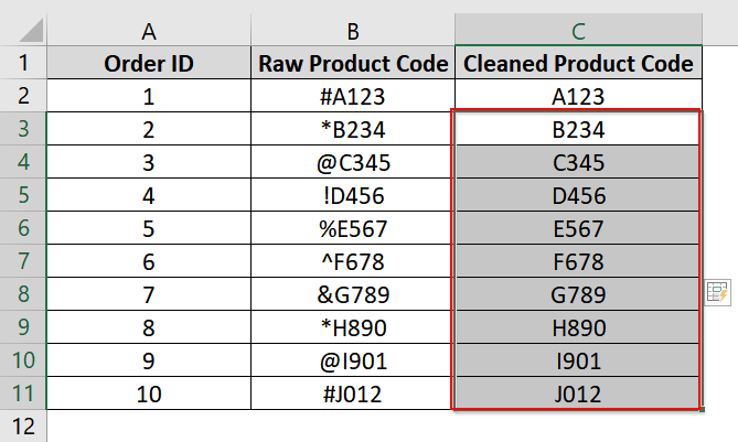
➤ Click on cell C3, and press Ctrl + E on your keyboard. Excel will detect the pattern and fill the rest of the column by removing the unwanted characters based on our example at C2.
Note:
➥ Flash Fill is available in Excel 2013 and later.
➥ This method only works when there’s a consistent pattern for Excel to follow.
➥ If Flash Fill does not activate automatically, you can enable it via:
File > Options > Advanced > Enable Flash Fill..
Combining LEFT and LEN Functions to Remove Last n Unwanted Characters
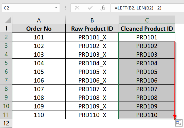
The combination of LEFT and LEN functions in Excel can remove a specific number of characters from the end of a text string. This is helpful when we are dealing with consistent suffixes like special symbols, redundant tags, or formatting codes in data fields like product IDs, codes, or serial numbers.
We have taken a dataset that contains Product IDs with an unwanted suffix “_X” at the end. We will use the combination of LEFT and LEN function to remove the last 2 characters from each ID.
Steps:
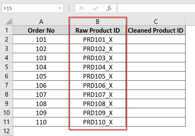
➤ Open your Excel dataset. We have Column B with unwanted values at the end like “PRD101_X“. We have inserted a new column (e.g., Column C) next to the original one and labeled it Cleaned Product ID.
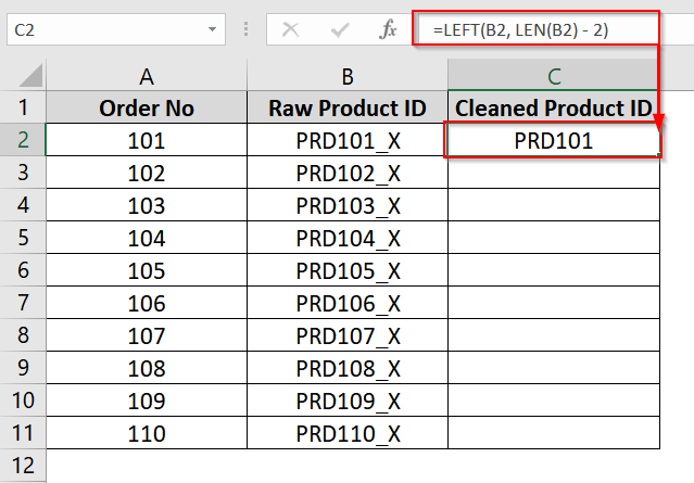
➤ In cell C2, type the following formula and click Enter:
=LEFT(B2, LEN(B2) – 2)
This formula tells Excel to take all characters from the beginning of the text except the last two. You will see the value “PRD101” returned, which is the original without “_X”.
➤ Click on the bottom-right corner of cell C2 and drag the fill handle down to copy the formula for the rest of the cells in Column C.
Note:
Change the “2” in LEN(B2) – 2 to match the number of characters you want to remove from the end.
Combining RIGHT and LEN Functions to Remove First n Unwanted Characters
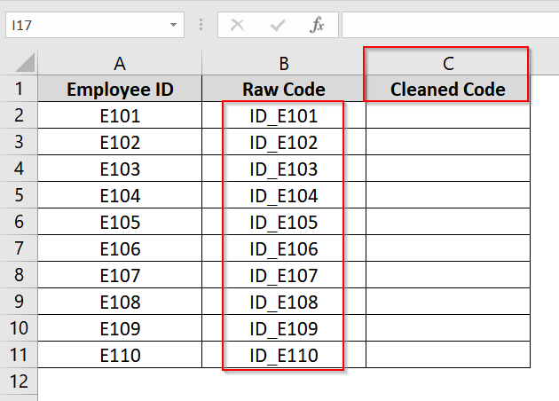
The combination of RIGHT and LEN functions in Excel can remove a specific number of characters from the start of a text string. It is useful when dataset entries have consistent prefixes, such as IDs with tags or codes starting with extra markers that need to be removed.
We have taken an example dataset that contains Raw Code with a prefix “ID_” that is unnecessary for further processing. We will use the combination of RIGHT and LEN to remove the prefix and retain the necessary part of the code.
Steps:
➤ Open up your dataset. We have Raw Code in Column B which contains unwanted characters. We have named column C as Cleaned Code where we will store the cleansed code after removing unwanted characters.
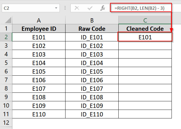
➤ In cell C2, type the following formula and click Enter:
=RIGHT(B2, LEN(B2) – 3)
This tells Excel to return all characters after the first 3 characters of cell B2. You will now see the result “E101” in cell C2
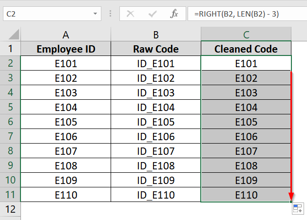
➤ Drag the fill handle (bottom-right corner of cell C2) down to apply the formula to other rows in Column C.
Note:
➥ Change the number 3 in the formula if your prefix has a different length.
➥ If the prefix isn’t consistent in length, consider using MID or TEXTAFTER functions instead.
Frequently Asked Questions (FAQs)
How do I remove unwanted text from a cell in Excel?
You can use the SUBSTITUTE function to replace the unwanted text with a blank. For example, =SUBSTITUTE(A1, “ID_”, “”) removes the “ID_” prefix.
How do I delete unnecessary characters in Excel?
Depending on the character, use one of the following functions:
- TRIM to remove extra spaces
- SUBSTITUTE for specific characters or text
- LEFT or RIGHT to chop off extra characters from start/end
How do I remove 3 digits from the left in Excel?
Use: =RIGHT(A1, LEN(A1) – 3). This removes the first 3 characters regardless of what they are.
How do I remove random characters in Excel?
Use a combination of SUBSTITUTE and CLEAN functions to remove known unwanted characters and non-printable symbols. You can also use Flash Fill to pattern-match and auto-correct.
Concluding Words
Removing unwanted characters in Excel doesn’t have to be manual or time-consuming. We have shown six methods that can do that easily. We have shown Excel’s built-in tools like Find and Replace, Flash Fill which you can use if you don’t want to use formulas or functions. And if you want to use formulas or functions you can use SUBSTITUTE , TRIM and other mentioned methods.