Duplicate data can be a major headache, especially when you need to ensure the accuracy of your information. While Excel’s built-in “Remove Duplicates” tool can help, but it often leaves one instance of the duplicate data behind. Sometimes, you might need to remove all records of a duplicate, leaving only the unique records. In this article, we will guide you through four different ways to remove both duplicates in Excel.
To remove both duplicates in Excel:
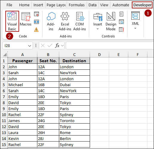
➤ Go to Developer > Visual Basic.
➤ In the VBA Editor, click Insert > Module.
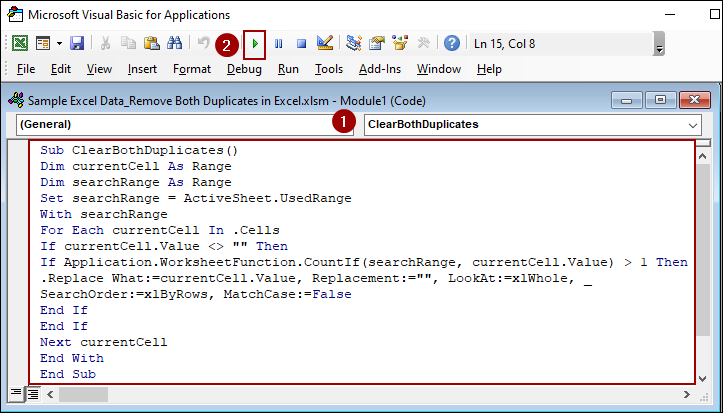
➤ Paste the below code and hit Run to remove both duplicates and collect unique data.
Sub ClearBothDuplicates()
Dim currentCell As Range
Dim searchRange As Range
Set searchRange = ActiveSheet.UsedRange
With searchRange
For Each currentCell In .Cells
If currentCell.Value <> "" Then
If Application.WorksheetFunction.CountIf(searchRange, currentCell.Value) > 1 Then
.Replace What:=currentCell.Value, Replacement:="", LookAt:=xlWhole, _
SearchOrder:=xlByRows, MatchCase:=False
End If
End If
Next currentCell
End With
End Sub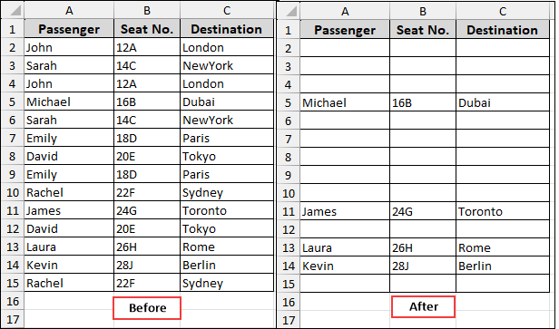
Using COUNTIF Function & a Helper Column to Remove Both Duplicates
In this method, we will use a helper column to identify which rows are duplicates. Then, use the COUNTIF function to count the occurrences of each value in a specific column. Lastly, we will filter the data to collect only the unique data.
For this example, we will use a dataset of passenger information, where some passengers have multiple entries.

➤ First, add a new column next to your data and name it “Helper Column”.
➤ In the first cell of the helper column (D2 in our example), enter the following formula, and drag down to fill.
=COUNTIF($A$2:$A$15,A2)=1
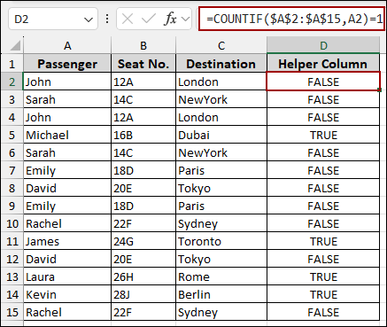
Thus, we will get TRUE for unique values and FALSE for duplicates.
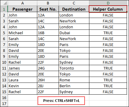
➤ Select any cell from the header row and press Ctrl + Shift + L to apply filters to all columns.
➤ Click the filter arrow in the “Helper Column” header.
➤ Uncheck FALSE and click OK.
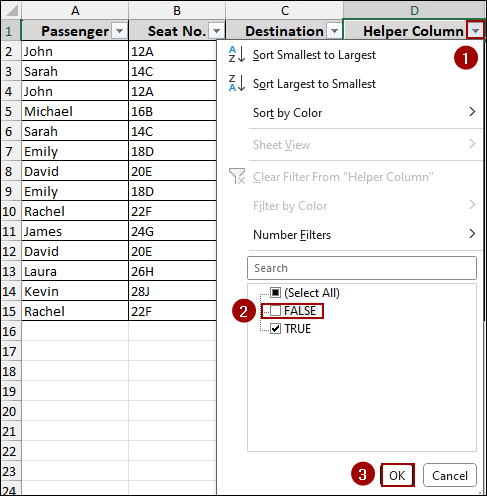
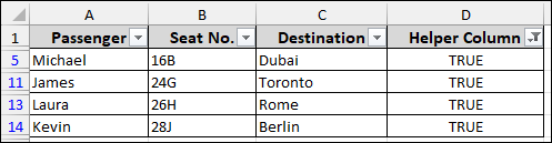
Finally, you will get the unique data, removing both duplicates in Excel.
Combination of IF and COUNTIF Functions
This is a variation of the previous method, but it gives you a more descriptive result in your helper column. Here, we will use the combination of IF and COUNTIF functions to understand which rows are duplicates.
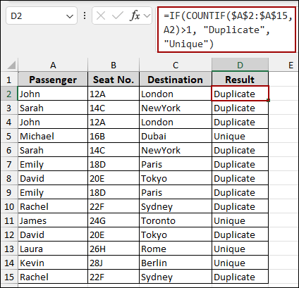
➤ Add a new column, in the first cell (D2), enter the formula, and drag down to fill.
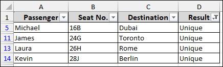
=IF(COUNTIF($A$2:$A$15,A2)>1,"Duplicate","Unique")
This way, each cell will now display either “Duplicate” or “Unique”.
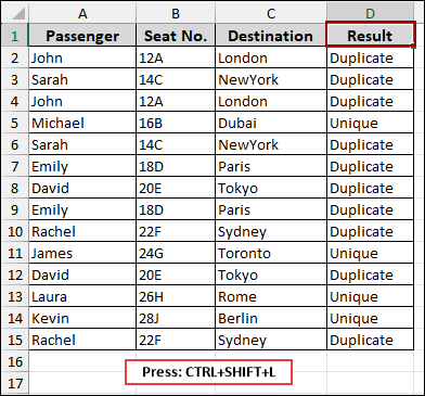
➤ Select any cell from the header and press Ctrl + Shift + L to apply filters.
➤ Click the filter arrow in the “Result” header.
➤ Uncheck “Duplicate” and click OK.
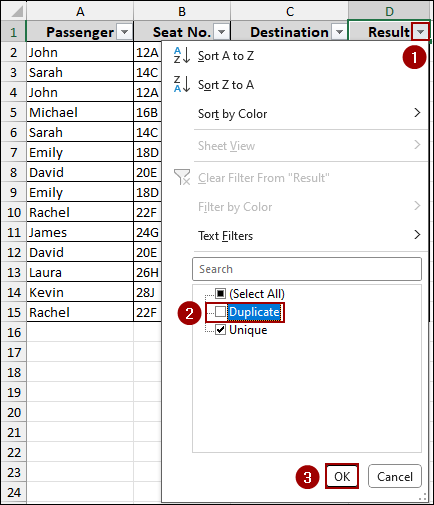
As a result, your data will display only the unique entries.
Applying Conditional Formatting
Conditional Formatting is a great tool to visually identify duplicates without using a helper column. First, highlight the data and then sort your data to group the duplicates for easy deletion.
Duplicate Values Feature
Here, we will use the Duplicate Values tool from Conditional Formatting to highlight duplicate values. Then we will sort the duplicates and remove the data.
➤ Select your data where you want to find duplicates.
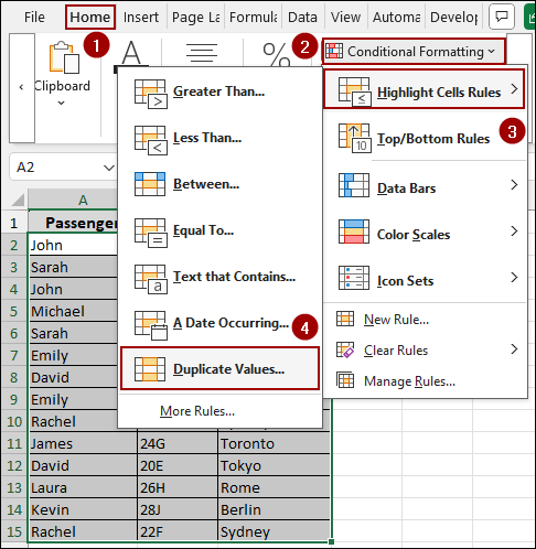
➤ On the Home tab, click Conditional Formatting > Highlight Cells Rules > Duplicate Values.
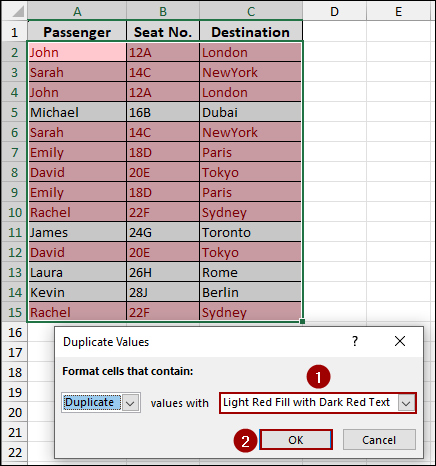
A dialog box will appear.
➤ Choose a format from the dropdown, such as Light Red Fill with Dark Red Text, and click OK.
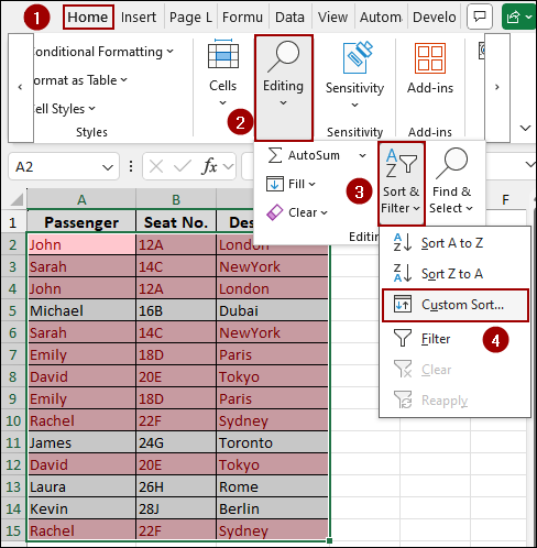
➤ Now that the duplicates are highlighted, select your data and go to Home > Editing > Sort & Filter > Custom Sort.
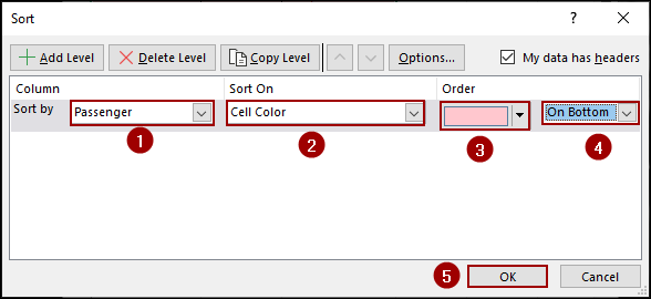
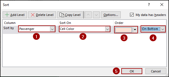
➤ In the “Sort” dialog box, set the following options.
Sort by: Select the column you applied conditional formatting to (“Passenger”).
Sort On: Choose Cell Color.
Order: Select the colored cell (e.g., the light red fill) and set it to On Bottom.
➤ Click OK.
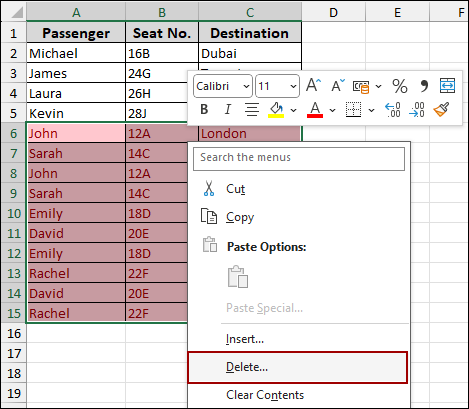
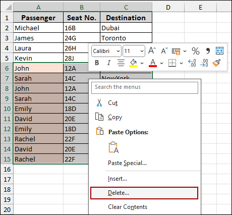
All the highlighted duplicate rows will now be at the bottom of your sheet.
➤ Select these rows and press the Delete option from the context menu.
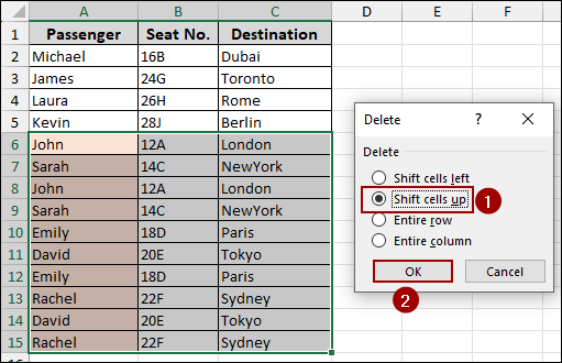
➤ Choose Shift cells up and hit OK.
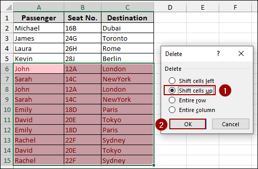
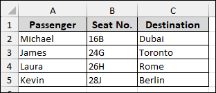
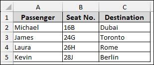
This way, we will get the unique data, removing both duplicates.
New Rule Feature
This method is similar to the previous one. Here, we will use a formula inside the New Formatting Rule window to highlight duplicates. Then, sort and delete the highlighted duplicates to get the unique values only.
➤ Select your data and click Conditional Formatting > New Rule.
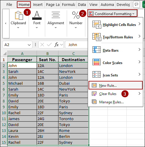
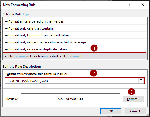
➤ Select “Use a formula to determine which cells to format” and enter the following formula.
=COUNTIF($A$2:$A$15,A2)>1
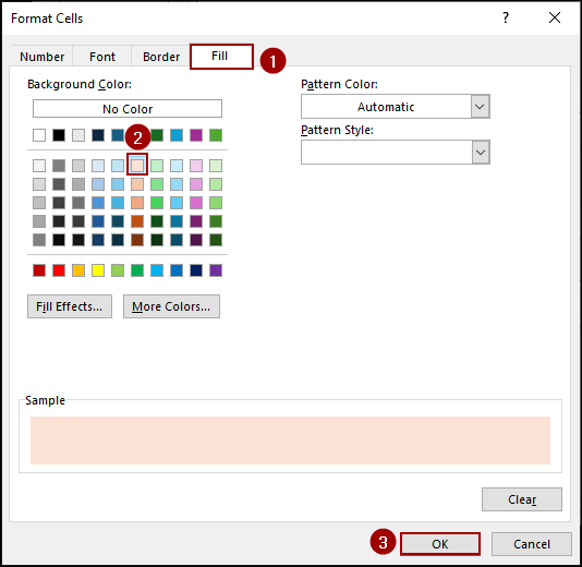
➤ Click Format.
➤ In the “Format Cells” dialog box, go to the Fill tab and choose a color to highlight the duplicates.
➤ Click OK.
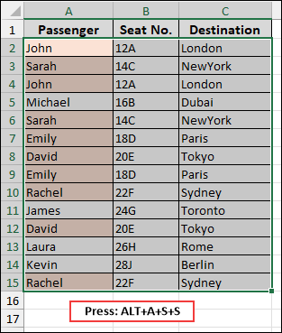
The duplicates will now be highlighted.
➤ Selecting the data, press Alt + A + S + S to open the Custom Sort window.
➤ In the “Sort” dialog box, set the following options.
Sort by: Select the column you applied conditional formatting to (“Passenger”).
Sort On: Choose Cell Color.
Order: Select the colored cell and set it to On Bottom.
➤ Click OK.
➤ Choose the highlighted duplicates from the bottom and click Delete from the context menu.
➤ Select Shift cells up and hit OK.
Thus, all the duplicates will be removed.
Using VBA Code to Eliminate Both Duplicates at Once
To remove both duplicates quickly with a press of a single click, you can use a VBA macro. Here, we will use a simple VBA code to find and remove all duplicate values from the selected column.
➤ Go to the Developer tab and click on Visual Basic.
➤ In the VBA editor, go to Insert > Module.
➤ Copy the following code into the new module window and hit Run.
Sub ClearBothDuplicates()
Dim currentCell As Range
Dim searchRange As Range
Set searchRange = ActiveSheet.UsedRange
With searchRange
For Each currentCell In .Cells
If currentCell.Value <> "" Then
If Application.WorksheetFunction.CountIf(searchRange, currentCell.Value) > 1 Then
.Replace What:=currentCell.Value, Replacement:="", LookAt:=xlWhole, _
SearchOrder:=xlByRows, MatchCase:=False
End If
End If
Next currentCell
End With
End Sub➧ For Each currentCell In .Cells: Loops through each cell within the defined search range.
➧ If currentCell.Value <> "" Then: Ensures that blank cells are skipped during the duplicate check.
➧ If Application.WorksheetFunction.CountIf(searchRange, currentCell.Value) > 1 Then: Checks if the current cell’s value appears more than once in the search range, meaning it is a duplicate.
➧ .Replace What:=currentCell.Value, Replacement:="", LookAt:=xlWhole, SearchOrder:=xlByRows, MatchCase:=False: Replaces all occurrences of the duplicate value in the range with an empty string.
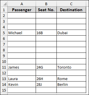
The macro will quickly run through your data and remove all instances of any duplicate values, leaving only the unique records.
Frequently Asked Questions
How is removing both duplicates different from removing normal duplicates?
The regular “Remove Duplicates” tool in Excel keeps the first occurrence of a value and deletes the rest, while removing both duplicates deletes all occurrences of repeated values.
Does the built-in “Remove Duplicates” button delete both duplicates?
No, the built-in tool removes only duplicate entries after the first occurrence. To remove both, you need a helper column, conditional formatting, or VBA.
What happens if my duplicates have extra spaces?
Excel treats values with trailing or leading spaces as different. You can use the TRIM function before checking for duplicates to avoid missing them.
Concluding Words
Above, we have explored several methods to remove both duplicates in Excel. Whether you prefer a simple formula, conditional formatting, or an automated VBA macro, these techniques can help you clean your data and ensure you are working with unique data only. If you have any further questions or need assistance with other Excel tasks, feel free to share them below.