Changing the number format in Google Sheets is a very handy skill. For example, you are making a sheet where you need to insert phone numbers, but the sheet is removing the zero. It happens if the number you are entering is in ‘number format.’ If you change the format to ‘text’ format, then Google Sheets will keep the leading zero, and you will get the full mobile number.
That is one use case. There are thousands of use cases for using the number format options in Google Sheets.
We have talked about the basic 4 methods on how to change the number format in Google Sheets in this article. Let’s explore them.
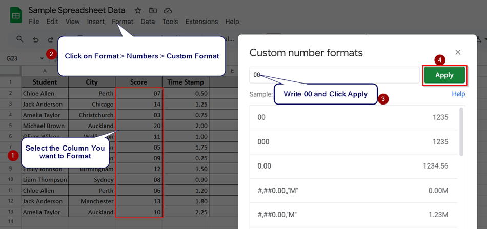
To customize numbers and make them 2-digit by adding leading zeros:
➤ Select all the numbers in the columns
➤ Go to the Format > Numbers > Custom Format
➤ Enter the rule: 00 and click Apply.
➤ This will display values like 5 as 05`.
There are many ways to format numbers in Google Sheets. Here, we will discuss 4 major methods with examples.
Conversion Between Number and Text in Google Sheets
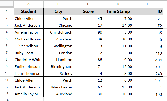
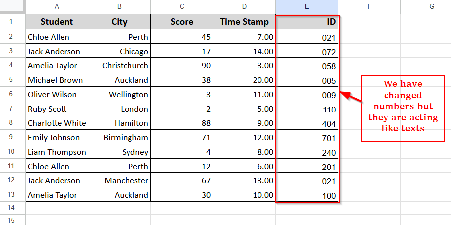
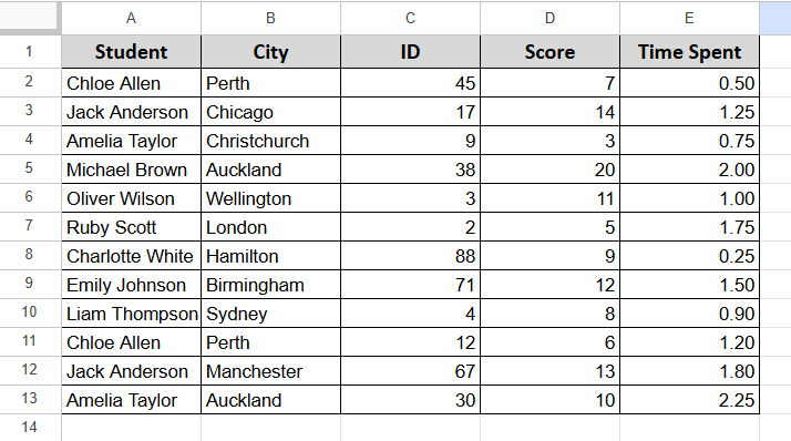
In the following dataset, we have a list of students in Column A and their cities in Column B. Their Exam Scores are in Column C, Time Stamps are in Column D, and the IDs are in Column E.
We’re going to do these things in the dataset:
- The ID column will be converted to plain text.
- Then again, change it back to the number format from plain text.
Convert Number to Text (Preserve Leading Zeros)
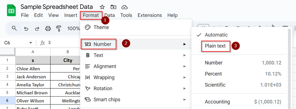
➤ Select the entire ID column.
➤ Go to the Format menu at the top.
➤ Hover over Number, then click Plain text.
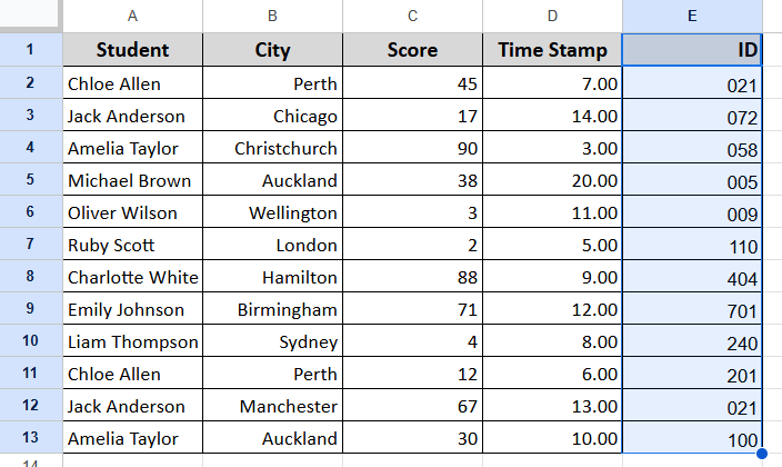
➤ Now go back to the column and manually retype IDs like 003, 017, or 071 if needed. Sheets won’t auto-correct them anymore.
And after applying plain text format, we can insert anything inside that column with a leading zero. It won’t auto-format. Here is the screenshot:
Convert Text to Number
Now we’ll convert the IDs stored as text back to the number format. Let’s follow the steps below:
➤ Select the ID column.

➤ Go to Format > Number > Automatic.
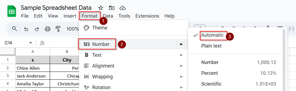
➤ If the values had been treated as text before, Sheets would now recognize them as proper numbers. So, there would be no leading zero now, and you can do calculations as you wish.
That was the process of converting a number to text and then text back to a number.
Conversion Between Decimal and Time
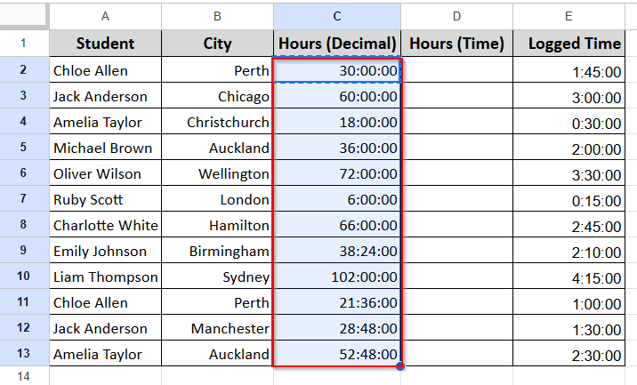
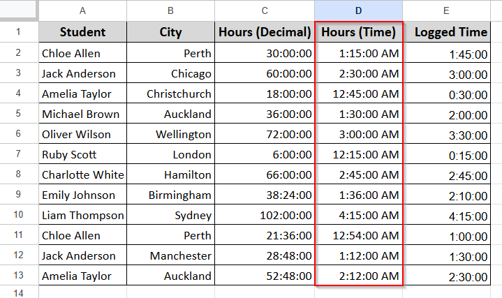
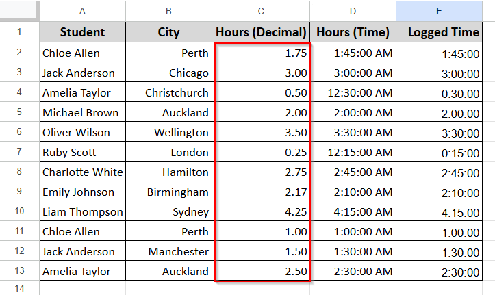
In this dataset, we have a list of students with their names in Column A and their cities in Column B. Column C shows how many hours each student spent on an assignment in decimal values. Column D will display those same values in time format.
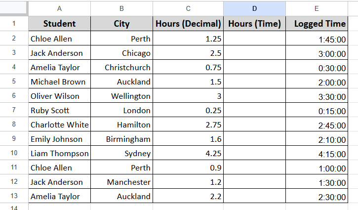
And the last Column E contains time-formatted values, and we will convert them back to decimals.
Convert Decimal to Time
Let’s turn the values in the Hours (Decimal) column into readable time.
Steps:
➤ Select the Hours (Decimal) column (Column C).
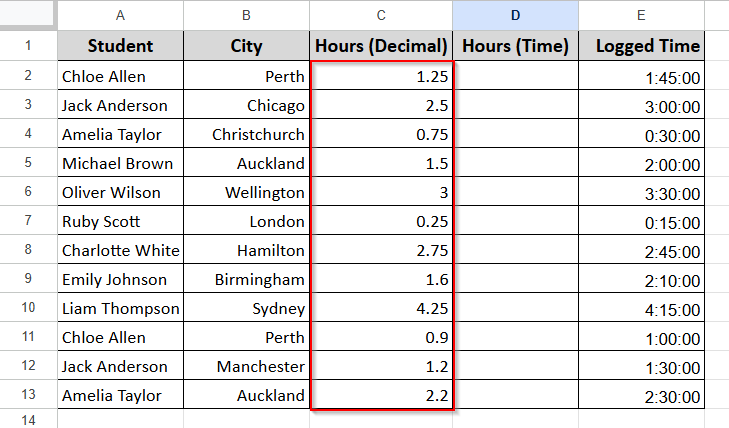
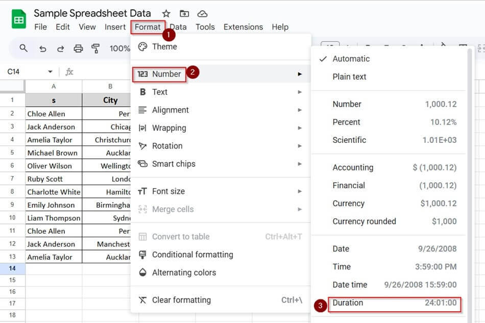
➤ Go to Format > Number > Duration.
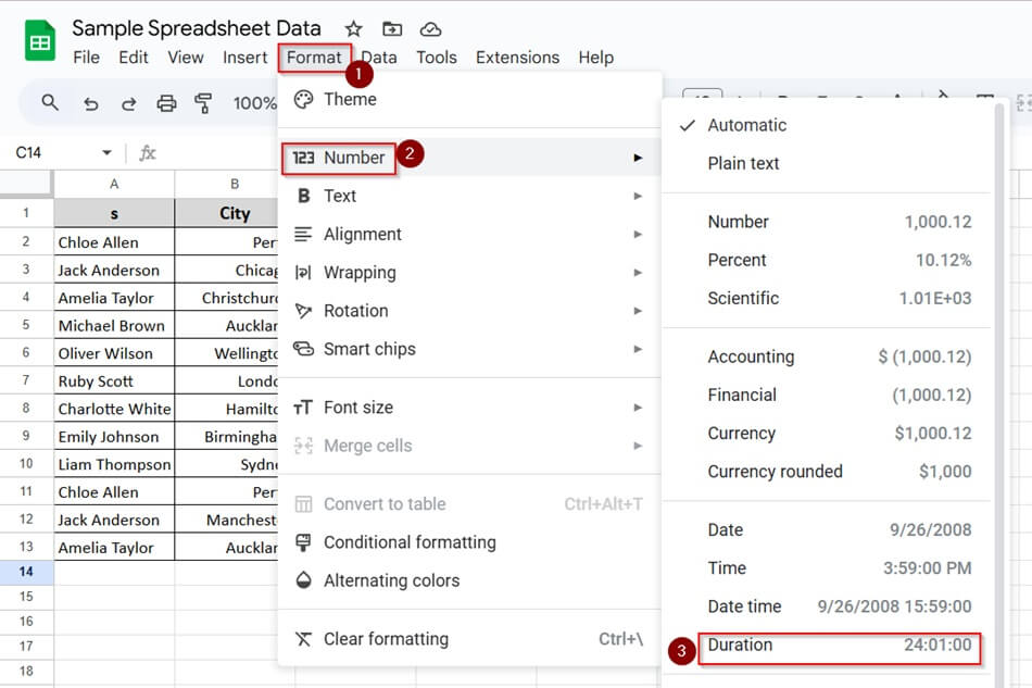
➤ Sheets will convert 1.25 into 30:00:00. But that’s not what we want to do.
➤ In Column D (Hours in Time), enter this formula in the first row:
This tells Sheets that your decimal represents part of a day (since time in Sheets is stored as a fraction of 24 hours).
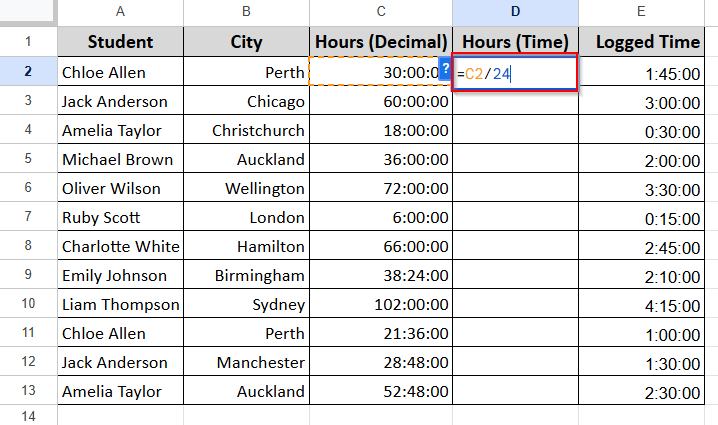
➤ Drag the formula down to fill the rest of Column D.
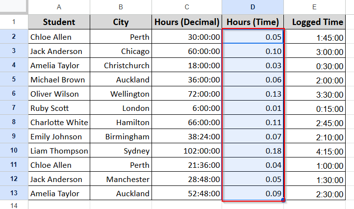
➤ Now format Column D by selecting- Format > Number > Time
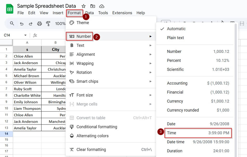
And here is your real time:
Convert Time to Decimal
Now let’s take the time-formatted values in Logged Time (Column E) and convert them into decimals.
Steps:
➤ In a new column (or reuse Column C if you want), type the formula:
=E2*24
This multiplies the time by 24 to get the total in hours.
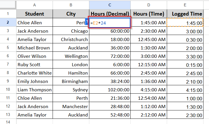
➤ But the output is not what we intended. It’s because it’s still in the duration form.
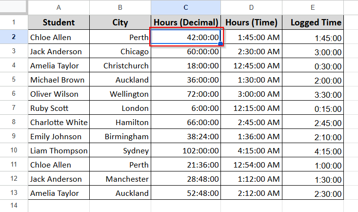
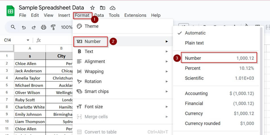
➤ Format the result using: Format > Number > Number or 0.00

Now we have a decimal number. Just drag it for the entire row, and you are done.
Conversion Between Number and Duration
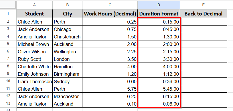
First, let’s describe the new dataset. This sheet tracks student work hours. You’ll see names in Column A, cities in Column B, and decimal hour values in Column C. These decimals show how long each student worked.
For example, 0.25 means 15 minutes, while 1.5 means an hour and a half.
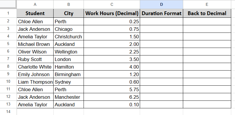
We’ll use Column D to display those hours as proper durations—like 1:30:00. Column E will then convert them back to decimals.
Convert Decimal to Duration
In the Work Hours (Decimal) column (Column C), we have regular numbers like 0.25, 1.5, or 5.75. These represent hours. But it’s tough to interpret them. For example, 0.25 means 15 minutes.
Let’s convert those into a clean duration format, so they look like 0:15:00, 1:30:00, etc.
Steps:
➤ In Column D (Duration Format), enter this formula in cell D2:
=C2/24
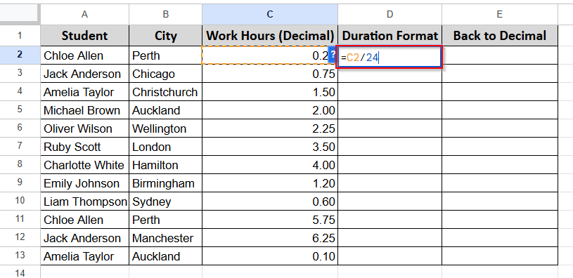
➤ Press Enter. Then drag the formula down the column.
➤ Now format Column D by going to Format > Number > Duration
Now you will get numbers in duration format in Column D
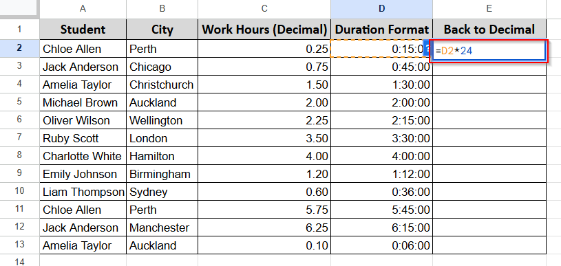
Convert Duration Back to Decimal
Now let’s flip it. You’ve got time values in Column D like 1:30:00 and 0:15:00. We want to turn them back into regular decimal numbers like 1.5 and 0.25.
But remember, don’t just change the format to “Number.” That won’t work. You need a formula.
Steps:
➤ In Column E (Back to Decimal), enter this formula in cell E2:
=D2*24
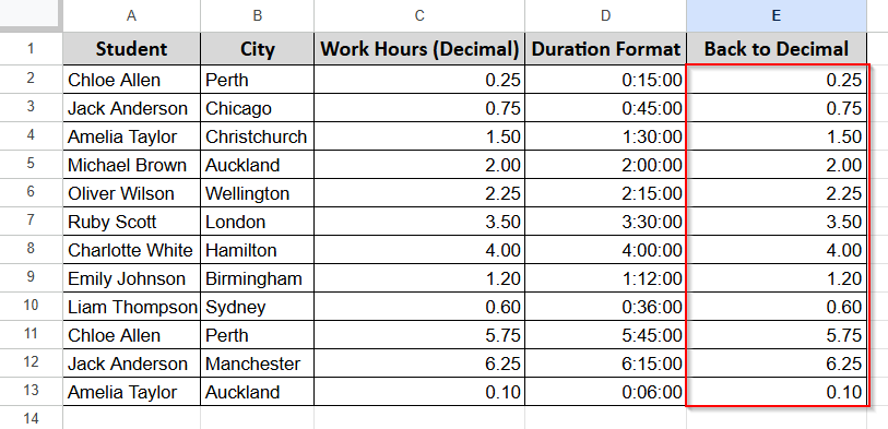
➤ Press Enter. Then drag the formula down the column.
➤ Format Column E by going to Format > Number > Number.
➤ Or use custom number format: 0.00
Here is the final output where you will get the original decimal in Column E:
Changing to Custom Number Format
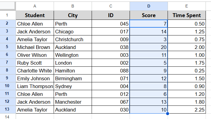
The following dataset lists students, their cities, IDs, scores, and time spent. The data is correct, but not easy to grasp the concept of the values shown.
To make it clearer:
- ID numbers like 3 or 9 should look like 003 or 009.
- Scores might show one decimal place, like 85.0
- The time spent column’s data is well organized.
So, we have to change the data in two columns (C&D). We will use custom number formats to do this.
Example 1: Add Leading Zeros to ID Column
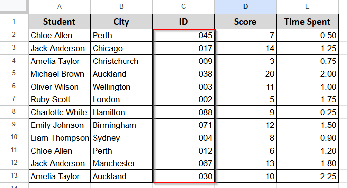
The ID column contains values like 3, 9, or 45. They’re all valid, but visually inconsistent. We want all IDs to appear as three-digit numbers—for example, 003, 009, 045.
This doesn’t change the value. It only changes how it looks.
Steps:
➤ Select the ID column (Column C).
➤ Go to Format > Number > Custom number format.
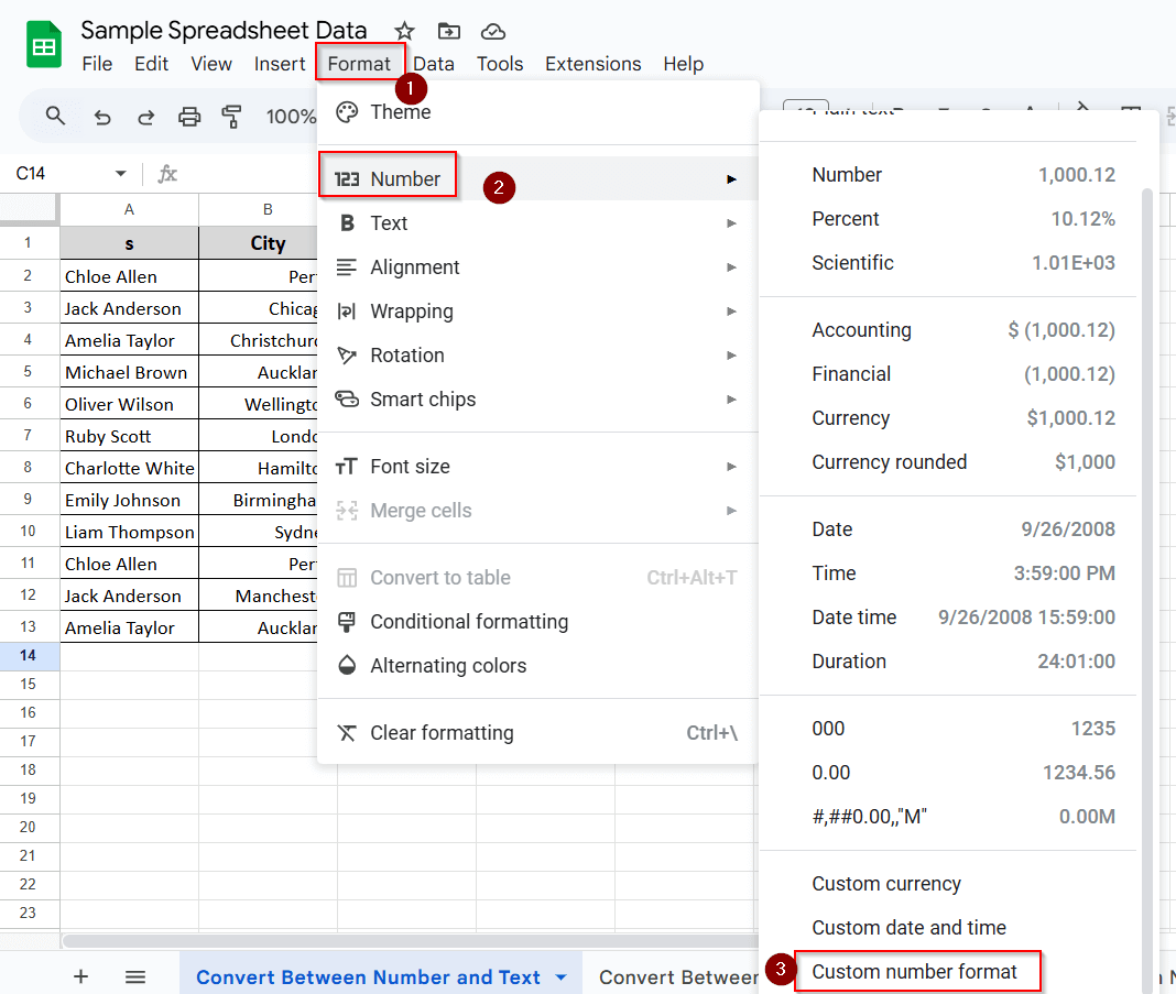
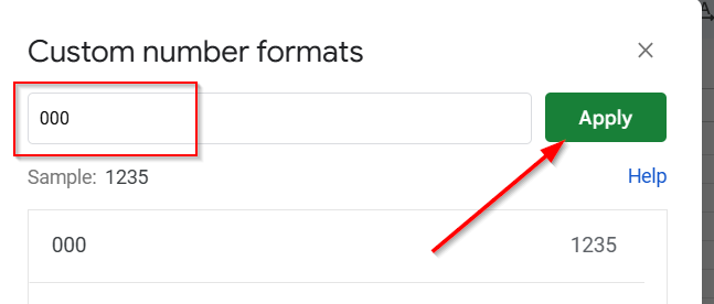
➤ In the field, type: 000
➤ Click Apply.
Here is the final output:
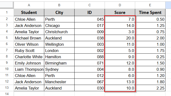
Example 2: Force One Decimal Place in Score Column
The Score column contains whole numbers—6, 14, 9. But in some contexts, especially with exams, you want to display all scores with one decimal place, even if the decimal is .0.
Steps:
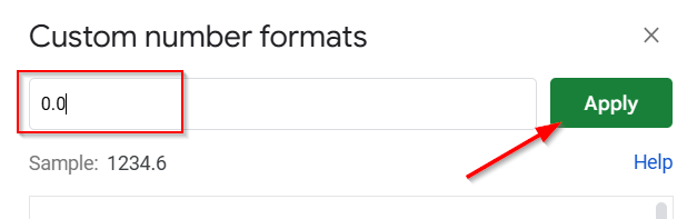
➤ Select the Score column (Column D).
➤ Go to Format > Number > Custom number format

➤ Type this format: 0.0
➤ Click Apply.
Here is the final output:
Example 3: Show Large Values in Millions
For this example, we will use a different datasheet. Here we will show you how you can convert a large number into a smaller one.
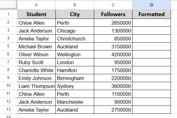
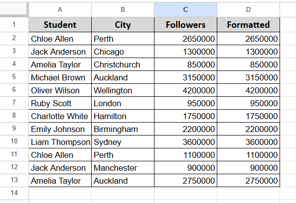
In this dataset, we have students’ names in Column A, their cities in Column B, and the number of followers they have on Instagram in Column C.
Our target is to make those numbers more readable by using the short format for numbers.
Steps:
➤ Copy and paste all numbers from Column C to Column D.
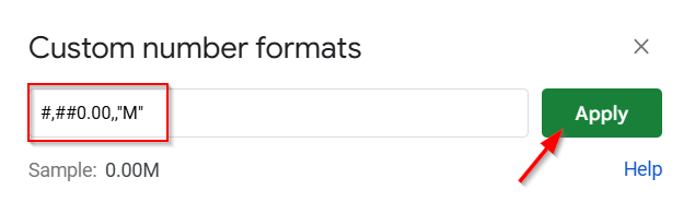
➤ Go to Format > Number > Custom number format
➤ Type this format: #,##0.00,,”M”
➤ Click Apply.
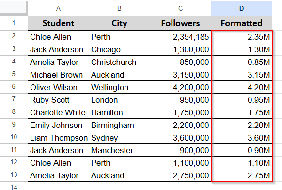
Now, let us explain how this format works.
➤ #,##0.00 makes sure your number will contain commas as thousand separators, where 0.00 confirms the number will have two decimal places.
➤ And the two commas after 0.00 make sure Google Sheets will divide the selected numbers by 1,000,000 (each comma is a division by 1,000).
➤At last, “M”, which refers to millions, ensures the letter M will appear just after the number.
Now, see the final output below in Column D:
Frequently Asked Questions
How do I fix a number format in Google Sheets?
It’s a formatting issue. You can select the cells and correct the formatting from the Format>Number menu. Or, you can use Format>Clear Formatting to clear the existing formatting.
How do I reset numbers in Google Sheets?
You should use clear formatting options to clear all types of formatting or reset numbers in Google Sheets. Use Format > Clear Formatting to clear the existing formatting.
How do I format automatic numbering in Google Sheets?
You can use the autofill feature. Here are the steps:
➤ First, write 1 in the first cell.
➤ In the cell below, type 2.
➤ Select both cells.
➤ Now drag the small blue square from the bottom-right corner downward.
Google Sheets will automatically fill the column with sequential numbers.
Concluding Words
In this article, you learned how to change the number format in Google Sheets. We have shown you 4 different methods and examples to elaborate on those methods. You get maximum liberty using the custom formatting method. But only use that if the default functions are not enough. The main goal is to streamline the working process.
And remember, formatting doesn’t affect your calculations. But they can make the sheet ugly if you don’t do it perfectly.