When your dataset contains positive and negative numbers, you can differentiate those numbers with colors so that anyone can easily get the value of the numbers at first glance.
In this article, we will learn how to make negative numbers red in Google Sheets using two different ways.
Steps to make negative numbers red:
➤ Select Conditional Formatting from the Menu bar.
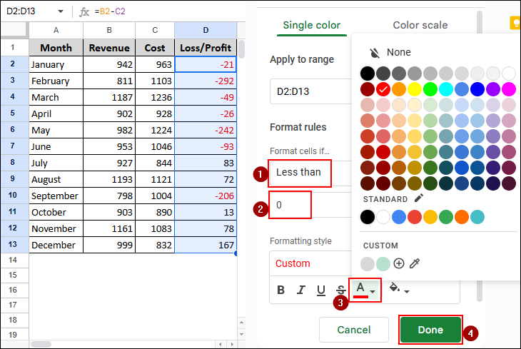
➤ Click on the “Format cells if” drop-down bar and select the Less than option.
➤ Write down 0 in the formula box.
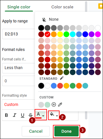
➤ Then change the color to red.
➤ Finally, click on Done to complete the process.
In this article, we will learn how to make negative numbers red in Google Sheets using conditional formatting and Custom number format.
Applying Conditional Formatting to Make Negative Numbers Red
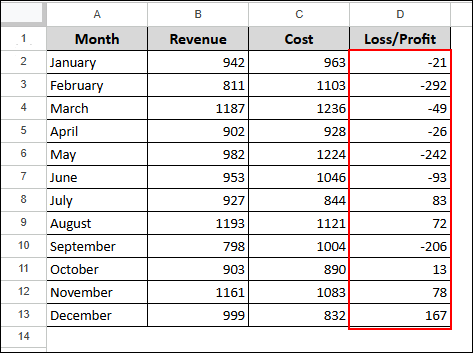
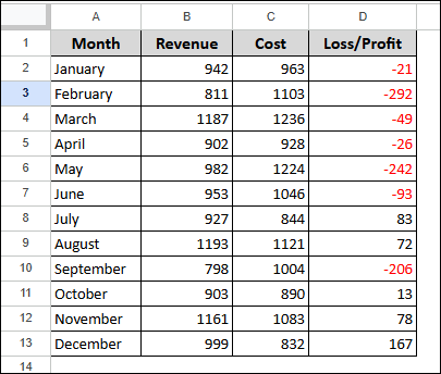
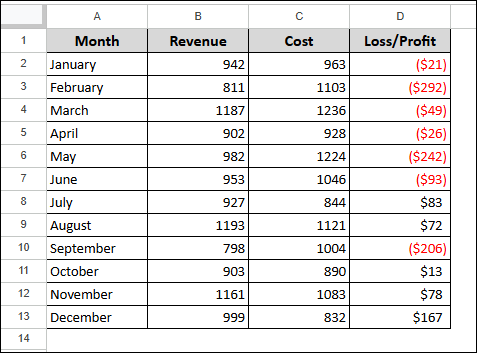
Let’s consider the dataset below, where we will calculate the yearly profit and loss of a company. The data is contained in Column D
Steps:
➤ Initially, select the dataset range. Here, the range is D2:D13.
➤ Then go to Format > Conditional Formatting from the Menu bar.
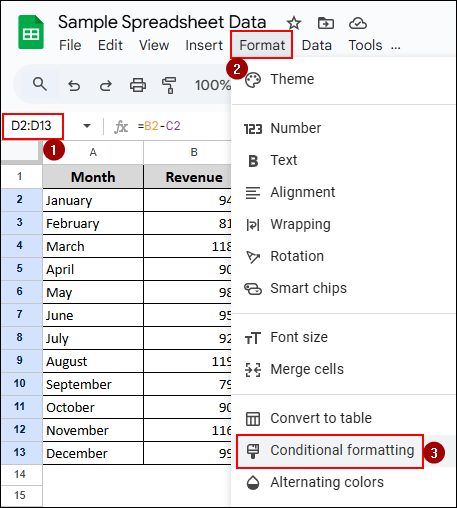
➤ After that, the Conditional format rules window will pop up.
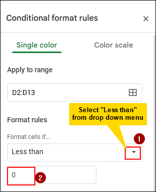
➤ Select Less than from the “Format cells if” drop-down bar and write down 0 in the formula bar.
➤ In the Formatting style option, select the Text Color as red and Fill color as white.
➤ Click on Done to complete the process.
➤ Here is the final output. The negative numbers are red.
Using the Custom Number Format Option
Steps:
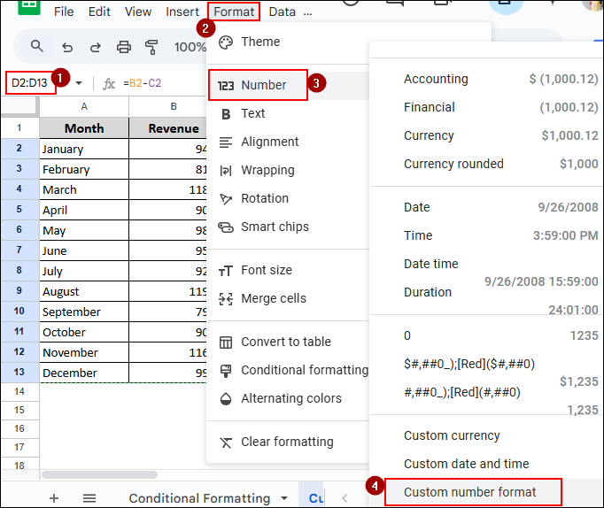
➤ Select the data range D2:D13 from the dataset.
➤ Go to the Menu bar and select Format > Number > Custom number format as shown.
➤ After that, the Custom number formats window will pop up.
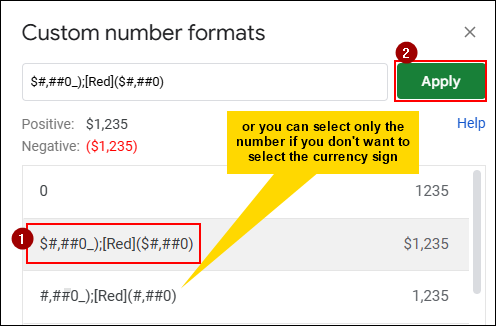
➤ Now, select the $#,##0_);[Red]($#,##0) option from the drop-down option below, or you can manually write it down in the box.
➤ There is another option without the $ sign. In case there are only numbers.
➤ Click Apply to complete the process.
➤ The final output is shown below. The profits are black and the losses are red.
Frequently Asked Questions
How to convert negative numbers to positive numbers in Google Sheets?
To convert your negative numbers to positive ones, follow the steps below:
➤ Initially, select a certain cell
➤ Then enter =ABS(Value) [here, the Value means, value of the cell, or write down the negative number you want to convert]
How do you make a negative number red?
To make a negative number red, follow the steps below:
➤ Select the cell and go to Home > Conditional Formatting > Highlight Cells Rules > Less than, then enter 0 in the box where the condition should be written.
➤ Select the red colour from the options and click OK to complete the process.
How to make a cell green if positive and red if negative in Google Sheets?
To make a positive number cell and a negative number cell red, you need advanced conditional formatting. Initially, you make the negative numbers red using the conditional formatting shown in this article, then you have to add another rule where you use the Greater than option in the “formula cells if” drop-down menu.
How do I make negative numbers not show up in Google Sheets?
If you don’t want the negative numbers to show up, then
➤ Click on a cell and enter [=(the cell reference of the negative number)*-1].
➤ Press Enter, and all the negative numbers will turn into positive ones.
Concluding Words
In this article, we learned how to make negative numbers red in Google Sheets using two different ways. One is using conditional formatting, and another is custom number format. Feel free to give us suggestions and feedback regarding this article.