When working across multiple spreadsheets, it’s often necessary to combine data from separate Google Sheets based on a shared column, like a common ID, email, or product name. Whether you’re consolidating inventory, syncing sales records, or cross-referencing customer details, joining sheets helps you unify your data for better analysis. In Google Sheets, this can be done using built-in formulas such as VLOOKUP and QUERY, or by applying automation with tools like Apps Script and third-party add-ons.
In this article, we will outline the most effective methods for joining two Google Sheets based on a common column, so you can save time, avoid manual errors, and build smarter spreadsheets.
Steps to join two Google Sheets based on a common column using VLOOKUP:
➤ Open your destination sheet where you want to pull the data.
➤ In a new column, use the formula:
=VLOOKUP(A2, IMPORTRANGE(“URL-of-source-sheet”, “Sheet1!A:B”), 2, FALSE)
➤ Replace A2 with the lookup value, and adjust the source range as needed.
➤ Click Allow Access when prompted to link sheets.
➤ The matching value from the second sheet will now appear in your destination sheet, automatically syncing updates.
Merge Data Using VLOOKUP and IMPORTRANGE
One of the simplest ways to join two Google Sheets based on a common column is by combining the VLOOKUP and IMPORTRANGE functions. This method pulls in matching values from a second spreadsheet using a shared key, like a Customer ID, and is ideal for merging columns like names, locations, or any reference data.
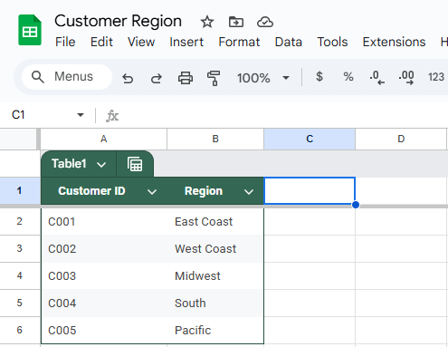
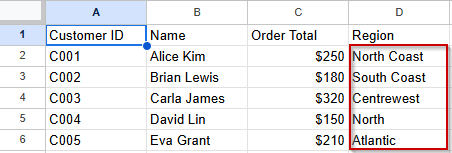
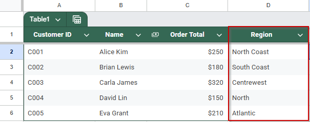
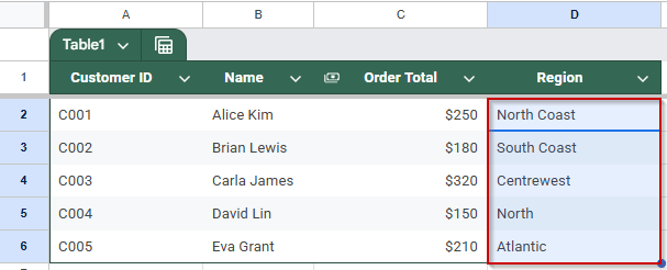
You’ll use this approach to bring the Region information from the Customer Region sheet into the Customer Orders sheet by matching on the Customer ID column.
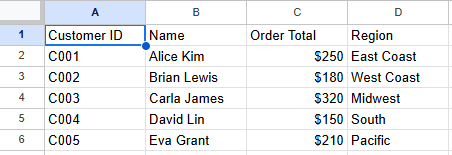
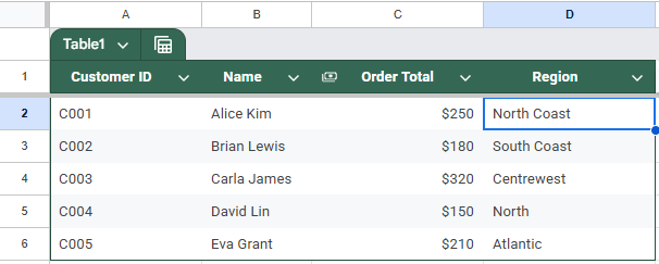
Customer Region dataset:
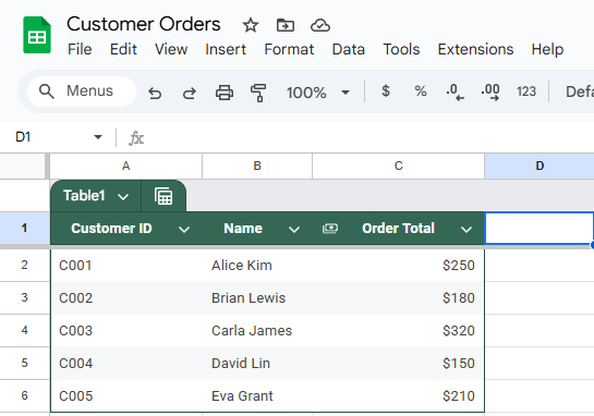
Customer Orders dataset:
Steps:
➤ Open Sheet 1 (Customer Orders) where you want to add the Region column.
➤ In a new column (e.g., Column D), label it Region.
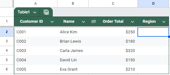
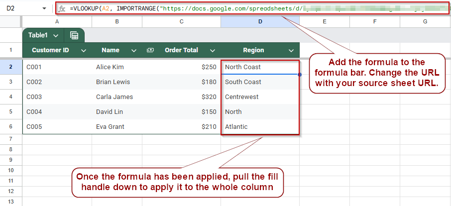
➤ In cell D2, enter the following formula:
=VLOOKUP(A2, IMPORTRANGE(“URL-of-Customer-Region-sheet”, “Sheet1!A:B”), 2, FALSE)
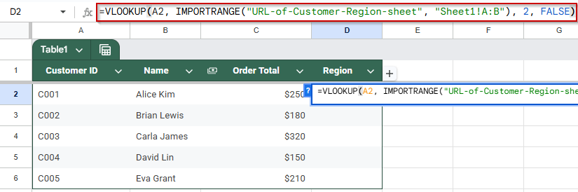
Replace “URL-of-Customer-Region-sheet” with the actual URL of Sheet 2.
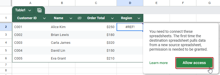
➤ When prompted, click Allow access to connect the sheets.
➤ Drag the formula down to apply it to all rows in the Region column.
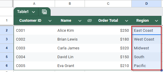
Each row in Sheet 1 will now show the corresponding Region from Sheet 2, based on the Customer ID.
Use the QUERY Function to Join Two Sheets Like a Database
If you’re comfortable with SQL-style logic, the QUERY function in Google Sheets offers a powerful way to join two datasets, especially when paired with IMPORTRANGE. This method behaves like a SQL JOIN, allowing you to merge sheets based on a shared column and retrieve selective fields.
It’s perfect when you want to extract specific columns from both sheets and create a unified table within one spreadsheet.
Steps:
➤ Open a new blank sheet where you want the joined data to appear.
➤ Now use the QUERY function to join and import the two different sheets using this formula (placed in A1):
=QUERY({IMPORTRANGE(“URL-of-Customer-Orders”, “Sheet1!A:C”), ARRAYFORMULA(VLOOKUP(INDEX(IMPORTRANGE(“URL-of-Customer-Orders”, “Sheet1!A:A”), ,1), IMPORTRANGE(“URL-of-Customer-Region”, “Sheet1!A:B”), 2, FALSE))}, “SELECT Col1, Col2, Col3, Col4 LABEL Col4 ‘Region'”)
➤ This creates a virtual joined table with columns: Customer ID, Name, Order Total, and Region.
The QUERY result will dynamically update when either source sheet is changed.
Use Google Sheets Add-Ons to Combine Sheets Without Formulas
If you prefer a no-code solution, Google Sheets add-ons like Merge Sheets or Sheetgo can simplify the process of joining two sheets based on a column. These tools are especially useful for users who manage large datasets or prefer a guided, interface-based method over formulas.
With just a few clicks, you can map key columns and merge rows across sheets, even across separate files.
Steps:
➤ Open your destination sheet (e.g., Customer Orders) in Google Sheets.
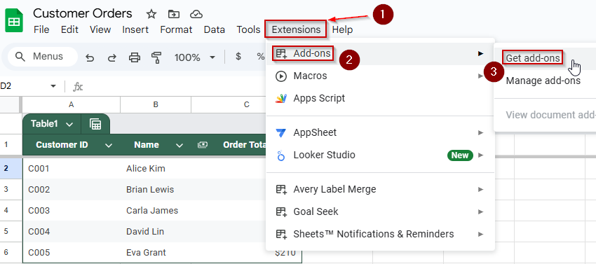
➤ Click on Extensions >> Add-ons >> Get add-ons
➤ Then search for “Merge Sheets” or “Sheetgo.”

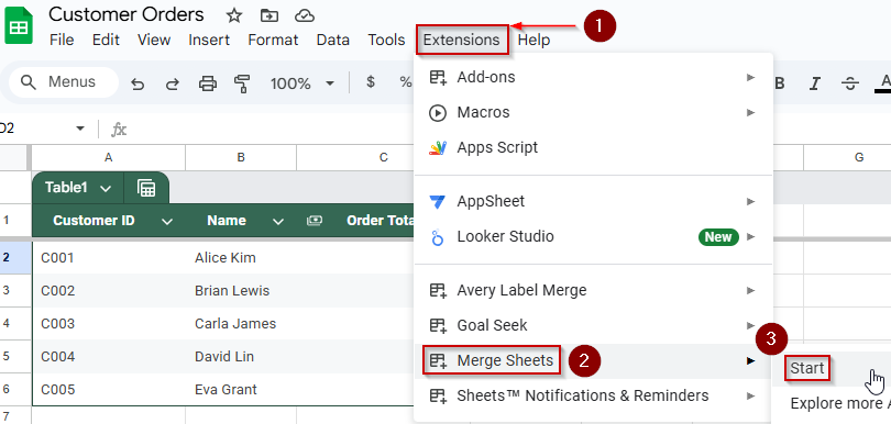
➤ Go to Extensions >> Merge Sheets >> Start.
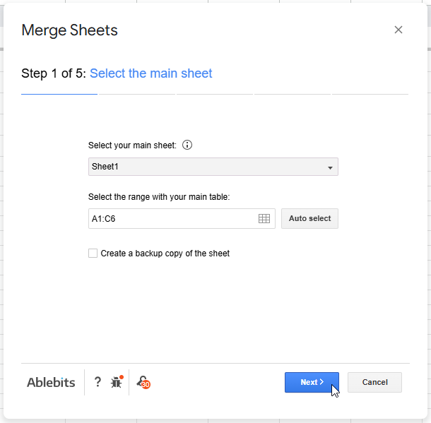
➤ Choose your primary sheet (Customer Orders) and then click on Next.
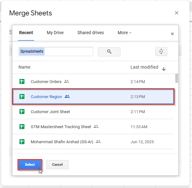
➤ Click on ‘Add files from a drive’ on the next page.

➤ Select your secondary sheet (Customer Region).
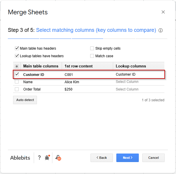
➤ Go to the next page and select the matching column (Customer ID) that the tool will use to join the data.
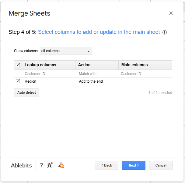
➤ Go to the next page and choose which columns to bring in (e.g., Region).
➤ Run the merge process. The add-on will append matching values into your destination sheet, either as new columns or a new tab.
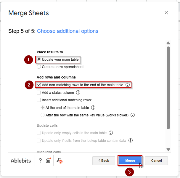
➤ The sheet should update once the merge process has been completed.
Automate Sheet Merging with Google Apps Script
For users comfortable with light coding, Google Apps Script offers a flexible way to automatically join two Google Sheets based on a column. This method is ideal when you need full control over how data is pulled, matched, and displayed in recurring tasks or workflows.
Using a script, you can programmatically match keys like Customer ID and populate data from one sheet into another without manual updates.
Steps:
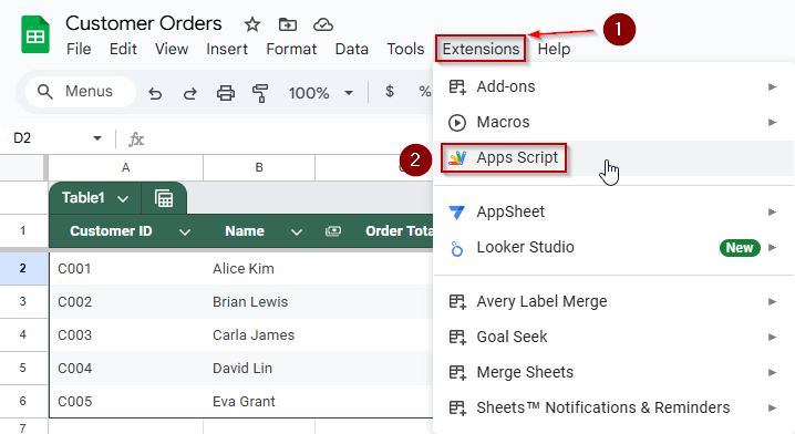
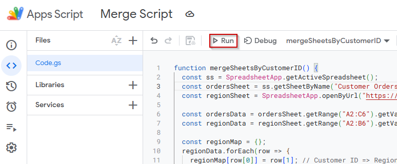
➤ Open your destination sheet (e.g., Customer Orders) and go to Extensions >> Apps Script.
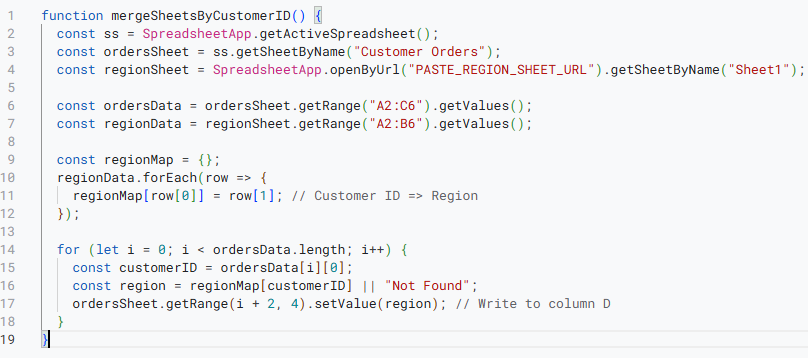
➤ Delete any placeholder code and paste the following script:
function mergeSheetsByCustomerID() {
  const ss = SpreadsheetApp.getActiveSpreadsheet();
  const ordersSheet = ss.getSheetByName("Sheet1");
  const regionSheet = SpreadsheetApp.openByUrl("PASTE_REGION_SHEET_URL").getSheetByName("Sheet1");
  const ordersData = ordersSheet.getRange("A2:C6").getValues();
  const regionData = regionSheet.getRange("A2:B6").getValues();
  const regionMap = {};
  regionData.forEach(row => {
    regionMap[row[0]] = row[1]; // Customer ID => Region
  });
  for (let i = 0; i < ordersData.length; i++) {
    const customerID = ordersData[i][0];
    const region = regionMap[customerID] || "Not Found";
    ordersSheet.getRange(i + 2, 4).setValue(region); // Write to column D
  }
}
➧ openByUrl("PASTE_REGION_SHEET_URL"): Connects to the external Google Sheet containing the lookup data. Replace "PASTE_REGION_SHEET_URL" with the actual URL of your second sheet.
➧ getRange("A2:C6"): Specifies the range in the destination sheet to read data from. Update this to cover your actual data range, including the shared key column (e.g., Customer ID).
➧ getRange("A2:B6"): Selects the range in the second sheet containing key-value pairs (e.g., Customer ID and Region). Adjust based on your sheet’s layout.
➧ regionMap Creates an object where the key is the Customer ID and the value is the corresponding Region. No changes needed unless your key-value structure differs.
➧ ordersSheet.getRange(i + 2, 4).setValue(region): Writes the matched Region into column D of the destination sheet. Change 4 to target a different column (e.g., 5 for column E).
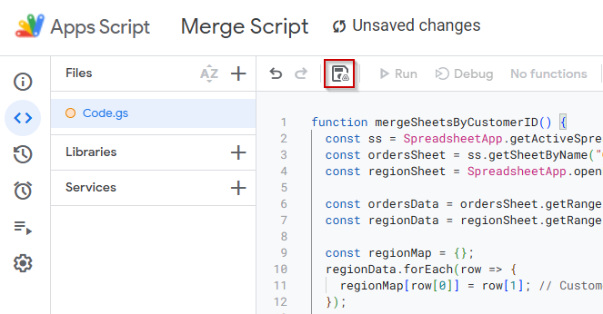
➤ Save the script by clicking on the floppy disk icon.
➤ Click the Run button to execute
➤ The Region values will be written next to the corresponding Customer IDs in Column D.
Combine Data with IMPORTRANGE and INDEX-MATCH
If you’re working across two different Google Sheets files, combining them based on a shared column like Customer ID becomes easy with the IMPORTRANGE and INDEX-MATCH combination. This method lets you pull in matching data from another sheet in real-time without needing any script or manual merging.
It’s a powerful option when you want to link sheets from separate files, maintain live connections, and avoid duplicating datasets.
Steps:
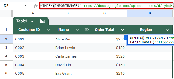
➤ In the primary sheet, use this formula to fetch the Region for a specific Customer ID in cell D2:
=INDEX(IMPORTRANGE(“PASTE_REGION_SHEET_URL”, “Sheet1!A2:B”), MATCH(A2, IMPORTRANGE(“PASTE_REGION_SHEET_URL”, “Sheet1!A2:A”), 0), 2)
➧ MATCH(A2, IMPORTRANGE("PASTE_REGION_SHEET_URL", "Sheet1!A2:A"), 0): Finds the row where the Customer ID in A2 appears in the imported list.
➧ INDEX(..., ..., 2): Returns the Region from the second column of the imported range.
➤ Press Enter.
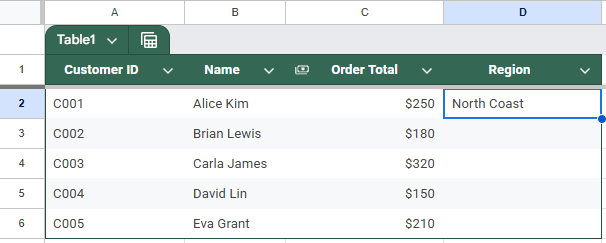
➤ Drag the formula down to fill in the results for the rest of your data.
This method creates a live link between two Google Sheets files, keeping your merged data automatically updated when the source file changes.
Frequently Asked Questions
Can I merge two sheets based on a common column without using Apps Script?
Yes, functions like VLOOKUP (with IMPORTRANGE), QUERY, and INDEX‑MATCH allow you to join data across sheets based on a shared key, without writing any code. These methods dynamically pull matching values from one sheet into another.
Why am I only getting the first matching result with VLOOKUP and IMPORTRANGE?
VLOOKUP always returns the first exact match. To retrieve multiple matches, use array or filtering techniques (e.g., FILTER on an IMPORTRANGE range), or switch to QUERY for SQL-style joins. A Reddit expert notes using FILTER or XLOOKUP combinations instead.
Do I need to grant access multiple times when using several IMPORTRANGE calls?
No. Google Sheets only requires you to Allow access once per spreadsheet link. After the initial confirmation, any subsequent IMPORTRANGE from the same source will work without additional prompts.
What do I do if the merged data doesn’t update automatically?
Most formula‑based merges (e.g., VLOOKUP+IMPORTRANGE, QUERY) update in real time. If they don’t, make sure:
➤ You’ve allowed access to the source sheet;
➤ You don’t have static copies or values instead of formulas;
➤ For Apps Script, you may need to set up Triggers to automate updates.
Wrapping Up
Joining two Google Sheets based on a column is a powerful way to combine data from different sources without duplication or manual entry. Whether you prefer formula-based solutions like VLOOKUP, INDEX-MATCH, and QUERY, or want more automation using Apps Script or add-ons, there’s a method for every skill level. With the right approach, you can build dynamic, connected spreadsheets that stay up-to-date and streamline your workflows across teams or departments.