How to Count Cells with Specific Text in Google Sheets

Whether you’re managing inventory, analyzing survey responses, or simply organizing lists, counting cells with specific text might be an important task on a regular basis. For example, you may want to count how many customers selected Yes in a feedback form, track how many times a product name appears in a sales list or monitor keywords in open-ended survey responses. Fortunately, you can simply count how many times a specific word appears in a range using the COUNTIF function.

This is the simplest and most common method to count cells with specific text in Google Sheets. In Google Sheets, the COUNTIF function counts the cells in a range based on a particular condition. But it’s not case-sensitive. So, Apple and apple will both be counted.

Below is the dataset where we have customer feedback along with product names, survey responses, order statuses, and sales regions. The data includes various case variations of the product Apple to illustrate text matching scenarios.

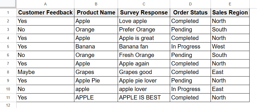
Now we’ll count the term “Apple” or “apple” from column B.

Steps:

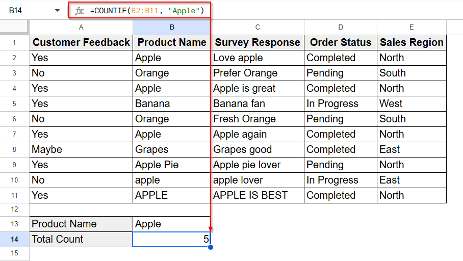
➤ Click a blank cell to insert the following formula with the COUNTIF function:

➤ Press Enter and you’ll see the total count of the term Apple from column B.

In Google Sheets, we can also use the COUNTIF function to count cells that contain partial matches, not just exact text. This is done by using wildcards such as asterisk (*), which allows you to search for text fragments within cells.

But still COUNTIF is case-insensitive here. It doesn’t differentiate between uppercase and lowercase. Depending on your goal, it will just count the word whether it’s an independent word or a part of a sentence or a phrase.

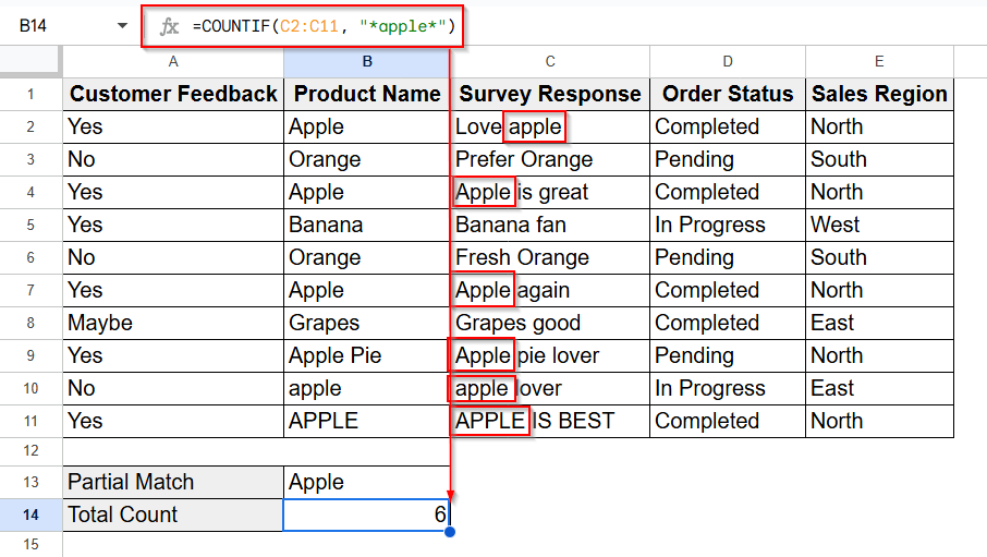
From column C, now we’ll find out how many times the word “apple” appears as a partial match. For example, “Apple pie” will also be counted based on the partial match “apple”.

Steps:

➤ Just as the previous method, identify the cell range and text to search for. For example C2:C11.
➤ Then click on a blank cell and  insert the formula with asterisk (*). The wildcard represents any number of characters before, after or middle of your keyword. For example:

Counting cells containing apple anywhere in the text:

And press Enter.

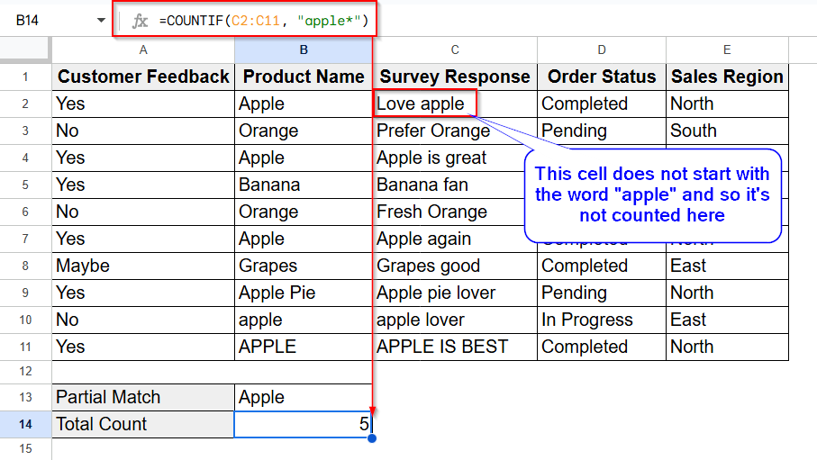
Counting cells starting with apple:

If we want to count how many cells in column C start with the word apple, then we have to use the following formula:

And after pressing Enter, you’ll the output as shown below:

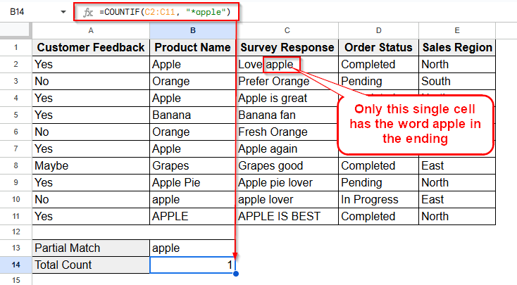
Counting cells ending with apple:

Now we’ll count how many cells in Column C are ending with the term “apple” and here the formula will be as follows:

After that, once you press Enter, the result will be seen as the image shows below.

This method is beneficial while counting all mentions of a keyword, even when it’s part of a sentence.

Unlike COUNTIF, Google Sheets allows case-sensitive counting using a combination of the SUMPRODUCT and EXACT functions. This method is useful when you need to differentiate between text like Apple and apple.

The EXACT function checks if two text strings are exactly the same, considering upper and lower case. It returns TRUE if they match exactly, and FALSE if they don’t. Then the double hyphen (–) converts TRUE/FALSE values into 1 and 0. Finally, SUMPRODUCT adds those values to give the final count. Here how it goes:

Now, as we’re going to see how this formula helps to count exact matches, we’ll choose a cell range B2:B11 from Column B. But since the EXACT function compares two pieces of text, the text should be included into a cell and we have to use cell reference this time.

Steps:

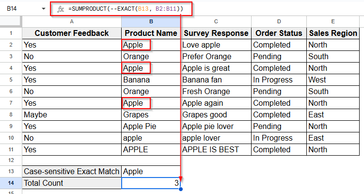
➤ Include the word Apple in the cell B13.
➤ Now, insert the following formula in B14:

➤ Press Enter and the formula will return the number of cells that exactly match the text in the cell B13, with the correct case.

If you want to count cells containing a specific word or phrase anywhere inside them and also want the match to be case-sensitive you can use a combination of FIND, ISNUMBER, and SUMPRODUCT functions.

FIND looks for the position of the search text in each cell and is case-sensitive. If it finds a match, it returns a number. If not, it returns an error. ISNUMBER converts successful matches to TRUE. The double hyphen — turns these into 1 (match) and 0 (no match). SUMPRODUCT adds them up for the final count.

Like the EXACT function, the FIND function also compares the targeted text with the words inside the targeted cell range and finds the matches. So, again we’ll have to include the text into a single cell. And as we’ll count partial matches, we’re going to use the C2:C11 cell range from the Column C.

Steps:

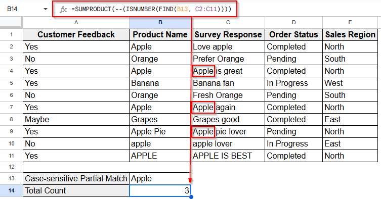
➤ Type the targeted word Apple inside the cell B13.
➤ Now insert the formula as follows:

➤ Press Enter. The result will show how many cells contain the exact case-sensitive keyword. For example, B13 contains Apple. So, this will not count apple or APPLE, only cells with Apple in that exact case will be counted as you can see in the image below.

In Google Sheets, to count cells containing multiple possible words, we typically combine multiple COUNTIF functions using addition or use COUNTA function with FILTER and REGEXMATCH for more complex patterns. This method sums the counts of each word separately.

But using multiple COUNTIF functions with addition may double-count cells containing both words. On the contrary, FILTER + REGEXMATCH can avoid duplicates while counting and is also case-sensitive. Compared to simple COUNTIF or EXACT, this approach handles multiple search terms but requires careful formula design to ensure accurate, non-overlapping results.

Using Multiple COUNTIF Functions

Till now, we counted the word Apple. Now we will count both the terms Apple and Orange from the Column C. So, here we’re going to combine two different COUNTIF functions together with an addition (+) sign.

Steps:

➤ Enter COUNTIF formula as it shows below:

➤ Press Enter and you’ll get the total count.

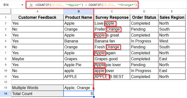
Here, if a cell contains both “Apple” and “Orange“, it will be counted twice. But as there’s no single cell with both the words, the answer is accurate here. So, using this method when overlapping is not a concern. Otherwise, here’s an alternative way to check in.

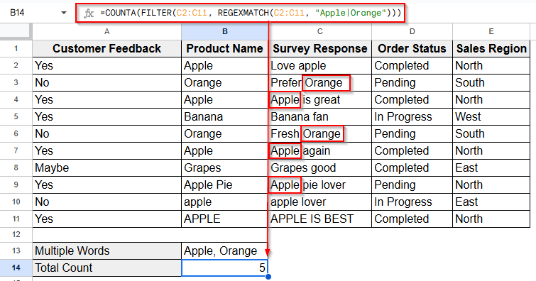
Using FILTER & REGEXMATCH Functions with COUNTA

In this method, we’ll be using the COUNTA function instead of the COUNTIF function. Generally, the COUNTA function counts how many cells in the range are not empty. But while Combining with FILTER and REGEXMATCH functions, it helps count how many cells have the specific text.

So, here we’ll also be using the Column C and count the words Apple and Orange while considering their case.

Steps:

➤ Insert the FILTER + REGEXMATCH formula as follows:

➤ Tap enter and you’ll get the correct count without double-counting.

Frequently Asked Questions

What if my range includes numbers or empty cells?

COUNTIF only evaluates text-based conditions. Empty cells won’t be counted unless the condition for them uses (“”) to count blanks.

Is there a way to count text across multiple sheets?

Yes, but you’ll need to reference each sheet individually:
=COUNTIF(Sheet1!A1:A100, “Apple”) + COUNTIF(Sheet2!A1:A100, “Apple”)

Why is my formula not working?

Common issues:

• Quotation marks are missing or curly instead of straight.
• The range is invalid (check for merged cells).
• Extra spaces in cell content (use TRIM() to clean them).

Concluding Words

Counting specific text in Google Sheets can be incredibly helpful when analyzing large datasets. Whether you need an exact match, a partial keyword, or a case-sensitive result, there’s a simple formula that gets the job done.

By mastering COUNTIF, EXACT, and SUMPRODUCT, you can turn Google Sheets into a smart, searchable database tailored to your needs.